Exercise 2: Define Boundary Conditions and Loads for the Seat Impact Analysis
In this exercise, you will define boundary conditions and load data for an LS-DYNA analysis of a vehicle seat impacting a rigid block.
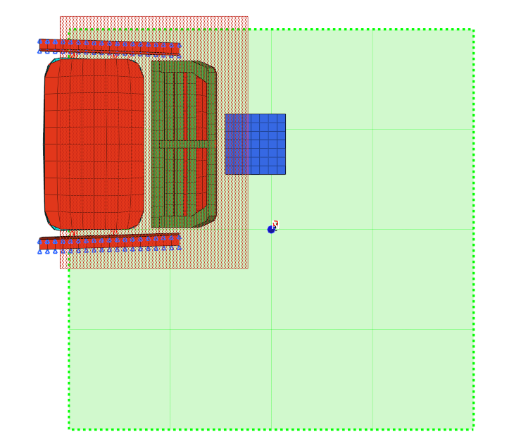
Figure 1.
Load the LS-DYNA User Profile
In this step, you will load the LS-DYNA user profile in Engineering Solutions.
- Start Engineering Solutions Desktop.
- In the User Profile dialog, set the user profile to LsDyna.
Retrieve the Engineering Solutions File
In this step, you will open the model file in Engineering Solutions.
-
Open the model file by completing one of the following options:
- Click from the menu bar.
- Click
 on the Standard toolbar.
Define Gravity Acting in the Negative Z-Direction
In this step, you will define gravity acting in the negative z-direction with *LOAD_BODY_Z.
-
In the Solver Browser, right-click and select and select Option Z from the context menu.
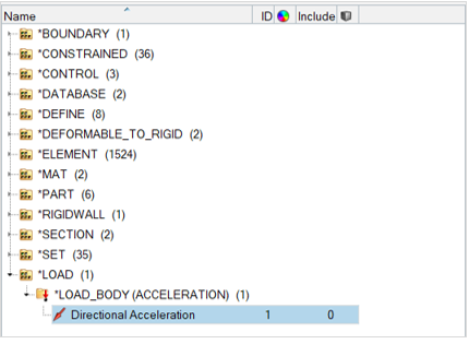
Figure 2.Engineering Solutions creates and opens a new load in the Entity Editor. -
Click LCID, and then click
curve.
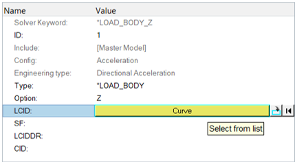
Figure 3.The Select Curve dialog opens. -
In the Select Curve dialog, select gravity
curve and then click OK.
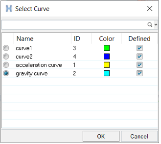
Figure 4.
Define the Seat Acceleration
In this step, you will define the seat acceleration with *BOUNDARY_PRESCRIBED_MOTION_NODE.
-
In the Solver Browser, right-click and select Create
*BOUNDARY *BOUNDARY_PRESCRIBED_MOTION (Accl) from the context menu.
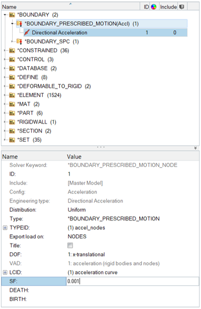
Figure 5.A new load collector is created and opened in the Entity Editor.
Export the Model
In this step, you will export the model to an LS-DYNA 971 formatted input file.
- From the menu bar, click .
- In the Export - Solver Deck tab, set File type to Ls-Dyna.
- In the File field, navigate to your working directory and save the file as seat_complete.key.
- Click Export.
Submit the Input File
In this step, you will submit the LS-DYNA Input File to LS-DYNA 971.
- From the Start Menu on your desktop, open the LS-DYNA Manager program.
- From the solvers menu, select Start LS-DYNA analysis.
- Load the seat_complete.key file.
- Click OK to start the analysis.
View the Results in HyperView
In this step, you will view the results in HyperView.
Save your work as a Engineering Solutions file.