In this tutorial the steps required to perform a buckling analysis using OptiStruct are covered.
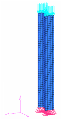
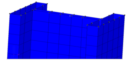
Figure 1 illustrates the structural model used for this
tutorial. Figure 1. Structural Model with Static Loads and Constraints Applied
Launch HyperMesh and Set the OptiStruct User Profile
Launch HyperMesh.
The User Profile dialog opens.
Select OptiStruct and click
OK.
This loads the user profile. It includes the appropriate template, macro
menu, and import reader, paring down the functionality of HyperMesh to what is relevant for generating models for
OptiStruct.
Open the Model
Click File > Open > Model.
Select the buckling.fem file you saved to
your working directory from the optistruct.zip file. Refer
to Access the Model Files.
Click Open.
The buckling.fem database is loaded
into the current HyperMesh session, replacing any
existing data.
Apply Loads and Boundary Conditions
Create Load Collectors
Create three load collectors (SPC, Static load and Buckling load).
Create the SPC load collector.
In the Model Browser, right-click and select Create > Load Collector from the context menu.
A default load collector displays in the Entity Editor.
For Name, enter SPC.
Click Color and
select a color from the color palette.
Create another load collector named Static load.
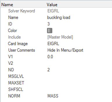
Create another load collector named buckling load.
For Card Image, select EIGRL.
For V1, enter 0.0.
For ND, enter 2.
This tells OptiStruct that you would like
to extract the first two buckling modes.
Figure 2.
Create Loads and Boundary Conditions
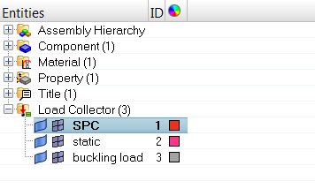
In the Model Browser, Load Collector folder, right-click on
SPC and select Make Current
from the context menu.
Figure 3.
From the menu bar, click BCs > Create > Constraints to open the Constraints panel.
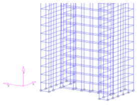
Select all of the nodes on the bottom face of the beam.
Click nodes > on plane.
Verify that the N1 selector is active, then click any three nodes on
the plane.
Click select entities.
All of the nodes on the plane are selected. Figure 4.
Deselect the degrees of freedom dof4 through
dof6.
Click create to create the necessary boundary
constraints.
Click return.
In the Model Browser, Load Collector folder, right-click on
Static load and select Make
Current from the context menu.
From the menu bar, click BCs > Create > Forces to open the Forces panel.
Select all of the nodes on the top face of the beam.
Figure 5. Nodes Selected for Application of Static Forces
In the magnitude= field, enter -10000.
Set the direction selector to z-axis.
Click create.
The forces display in the modeling window.
Click return.
Create a Load Step
The last step in establishing boundary conditions is the creation of a subcase.
Create the Linear load step.
In the Model Browser, right-click and select
Create > Load Step from the context menu.
A default load step displays in the Entity Editor.
For Name, enter Linear.
Set Analysis type to Linear Static.
For SPC, click Unspecified > Loadcol.
In the Select Loadcol dialog, select
SPC and click
OK.
For LOAD, click Unspecified > Loadcol.
In the Select Loadcol dialog, select
Static load and click
OK.
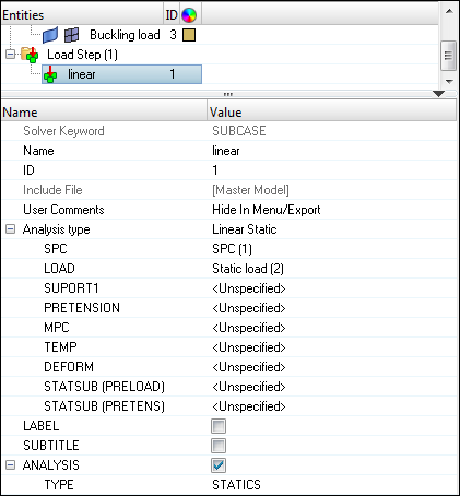
Figure 6.
Create the Buckling load step.
In the Model Browser, right-click and select
Create > Load Step from the context menu.
A default load step displays in the Entity Editor.
For Name, enter Buckling.
Set Analysis type to Linear buckling.
For METHOD(STRUCT), click Unspecified > Loadcol.
In the Select Loadcol dialog, select
Buckling load and click
OK.
For STATSUB(BUCKLING), click Unspecified > Loadcol.
A STATSUB card allows for the selection of a linear static subcase for
buckling analysis.
In the Select Loadcol dialog, select
Linear and click
OK.
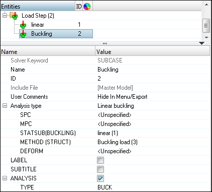
Figure 7.
Submit the Job
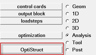
From the Analysis page, click the OptiStruct
panel.
Figure 8. Accessing the OptiStruct Panel
Click save as.
In the Save As dialog, specify location to write the
OptiStruct model file and enter
buckling for filename.
For OptiStruct input decks,
.fem is the recommended extension.
Click Save.
The input file field displays the filename and location specified in the
Save As dialog.
Set the export options toggle to all.
Set the run options toggle to analysis.
Set the memory options toggle to memory default.
Click OptiStruct to launch
the OptiStruct job.
If the job is successful, new results files
should be in the directory where the buckling.fem was written. The buckling.out file is a good place to look for error messages that could help
debug the input deck if any errors are present.
The default files written to the directory are:
buckling.html
HTML report of the analysis, providing a
summary of the problem formulation and the analysis results.
buckling.out
OptiStruct output file containing specific
information on the file setup, the setup of your optimization problem,
estimates for the amount of RAM and disk space required for the run,
information for each of the optimization iterations, and compute time
information. Review this file for warnings and errors.
buckling.h3d
HyperView binary results file.
buckling.res
HyperMesh binary results file.
buckling.stat
Summary, providing CPU information for each step during analysis
process.
View the Results
OptiStruct gives you contour information
for all of the loadsteps that were run. This section describes the process for
viewing those results in HyperView.
View Linear Load Step Results
From the OptiStruct panel, click the
HyperView icon.
HyperView launches with the
buckling.fem file which contains
the model and the results.
Use the drop-down Subcase selector to change the analysis that you are
reviewing in the current window.
Figure 9.
In the Results Browser, select Subcase 1 -
Linear.
On the Results toolbar, click to open the
Contour panel.
Select Element Stresses (2D and 3D) as the Result type
and set the sub type to von Mises.
Click Apply.
This should show the contour of von Mises stress.
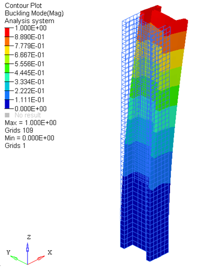
View Buckling Load Step Results
Click Clear Contour from the Result display control
panel.
In the Results Browser, click Subcase 2 -
Buckling and make sure the simulation is for Mode
1.
Click the Deformed panel toolbar .
Under Deformed shape, enter a value of 10.
Under Undeformed shape, for Show, select Wireframe from
the drop-down list.
Figure 10.
Click the Start/Pause Animation icon to view the animation.
 to open the
Contour panel.
to open the
Contour panel.
 .
.
 to view the animation.