OS-T: 1085 Linear Steady-state Heat Convection Analysis
This tutorial performs a heat transfer analysis on a steel pipe.
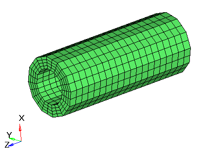
Figure 1. Model Review
Launch HyperMesh and Set the OptiStruct User Profile
Import the Model
-
Select the Files icon
 .
A Select OptiStruct file browser opens.
.
A Select OptiStruct file browser opens.
Set Up the Model
Create Thermal Material and Properties
-
Enter the following values for the material, steel, in the Entity Editor.
- [E] Young's modulus
- 2.1 x 10¹¹ Pa
- [NU] Poisson's ratio
- 0.3
- [RHO] Material density
- 7.9 x 10³ Kg/m3
- [A] Thermal expansion coefficient
- 1.0 x 10⁻⁵ / °C
- [K] Thermal conductivity
- 73W / m °C
- [H] Heat transfer coefficient
- 40W / m2 °C
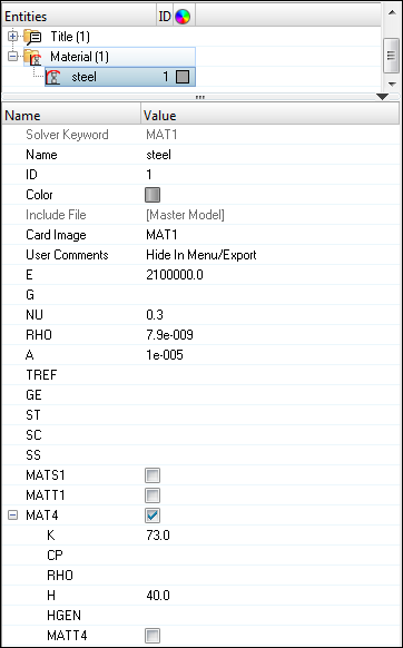
Figure 2. Material Entity EditorA new material, steel, is created with both structural and thermal properties.
Link Material and Property to Existing Structure
Apply Thermal Loads and Boundary Conditions
In this exercise the thermal boundary conditions are applied on the model and saved in a predefined load collector spc_temp. A predefined node 4679 specifies the ambient temperature. A predefined node set node_temp contains the nodes on the inside surface of the pipe.
Create Temperature on the Inner Surface of the Pipe
-
Click the Card edit icon
 .
.
Create Ambient Temperature
-
Click the Card edit icon .
-
In the field of D, enter 20.0.
The temperature boundary conditions are created, as shown below.
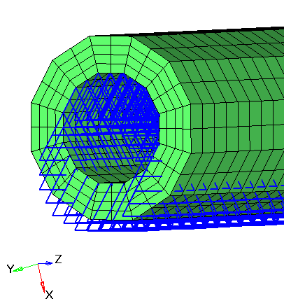
Figure 3. Thermal Boundary Conditions
Create CHBDYE Surface Elements
-
Select 4 nodes on the surface face of a solid element, as shown below.
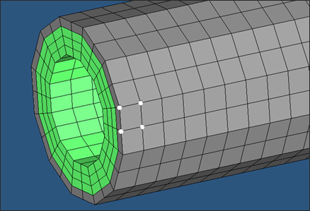
Figure 4. Selected Surface Nodes on the Solid Element Outside the Pipe -
Click add.
This adds the CHBDYE surface elements to the solid elements on the outer surface following the same side convention, as shown below.
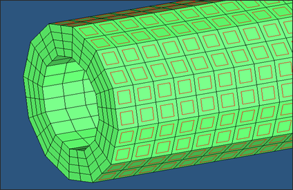
Figure 5. Surface Elements on the Outer Layer of the Pipe
Define Convection Boundary Condition to Surface Elements
-
Click the Card Edit icon .
-
Click TA1 and input the ambient node ID
4679, as shown below.
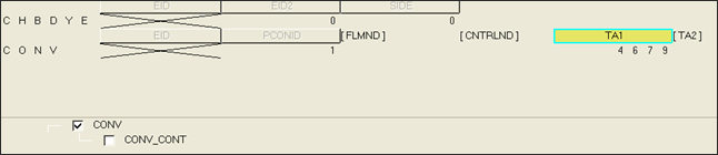
Figure 6. Define the Convection Boundary Condition
Create Heat Transfer Load Step
Submit the Job
-
From the Analysis page, click the OptiStruct
panel.
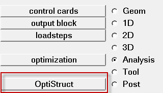
Figure 7. Accessing the OptiStruct Panel
View the Results
Gradient temperatures and flux contour results for the steady-state heat conduction analysis and the stress and displacement results for the structural analysis are computed from OptiStruct. HyperView will be used to post process the results.
-
On the Results toolbar, click
 to open the
Contour panel.
to open the
Contour panel.
-
Click Apply.
You may have to use Edit Legend in the Contour panel to get the contour. Both temperature and flux contour plots are shown in Figure 8.
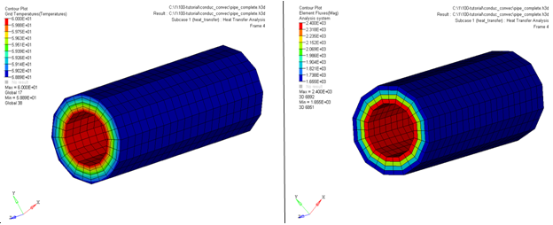
Figure 8. Results of Heat Transfer Analysis