OS-T: 1090: Linear Transient Heat Transfer Analysis of an Extended Surface Heat Transfer Fin
This tutorial outlines the procedure to perform a linear transient heat transfer analysis on a steel extended-surface heat transfer fin attached to the outer surface of a system generating heat flux (Example: IC engine). The extended surface heat transfer fin analyzed in this tutorial is one of many from an array of such fins connected to the system.
The fins draw heat away from the outer surface of the system and dissipate it to the surrounding air. The process of heat transfer out of the fin depends upon the flow of air around the fin (free or forced convection). In the current tutorial, the focus is on transient heat transfer through heat flux loading and free convection dissipation.
An extended surface heat transfer fin made of steel is illustrated in Figure 1. To meet certain structural design requirements, the fin is bent at 90° at approximately a quarter of its length.
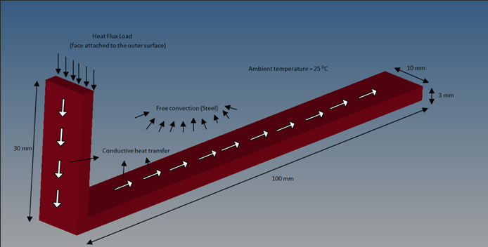
Figure 1. Extended Surface Heat Transfer Fin for Convective and Conductive Transient Heat Transfer
- The latest version of HyperMesh, HyperView and OptiStruct software installations. Transient heat transfer analysis is available only in HyperMesh version-12.0.110, HyperView version-12.0.110 and OptiStruct version-12.0.202 and later.
- The heat_transfer_fin.fem solver deck is available from the
optistruct.zip file. Refer to Access the Model Files.
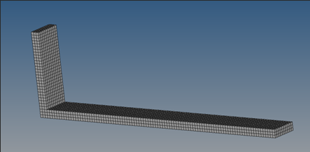
Figure 2. Heat Exchanger Fin Model for Transient Heat Transfer Analysis
Linear transient heat transfer analysis can be used to calculate the temperature distribution in a system with respect to time. The applied thermal loads can either be time-dependent or time-invariant; transient thermal analysis is used to capture the thermal behavior of a system over a specific period in time.
- Heat capacity matrix
- Conductivity matrix
- Boundary convection matrix due to free convection
- Temperature derivative with respect to time
- Unknown nodal temperature
- Thermal loading vector
The differential equation (Equation 1) is solved to find nodal temperature at the specified time steps. The difference between Equation 1 and the steady-state heat transfer equation is the term, that captures the transient nature of the analysis.
Steady-state heat transfer analysis, generally, is sufficient for a wide variety of applications. However, in situations where the system properties vary significantly over time the transient nature of heat transfer must be considered. Some examples are the relatively slow heating up of airplane gas turbine compressor disks compared to the turbine casing leading to aerodynamic issues during takeoff or the analysis of the time taken for the onset of frostbite in fingers or toes.
Launch HyperMesh and Set the OptiStruct User Profile
Import the Model
-
Select the Files icon
 .
A Select OptiStruct file browser opens.
.
A Select OptiStruct file browser opens.
Set Up the Model
Create Thermal Material and Property
-
Enter the following material property values for the MAT4
Data Entry.
- [K] Thermal Conductivity
- 7.3 x 10⁻²W/mm °C
- [CP] Heat Capacity at constant pressure
- 508J/Kg °C
- [RHO] Density of the material
- 7.9 x 10⁻⁶Kg/mm3
- [H] Coefficient of heat transfer
- 4 x 10⁻⁵W/mm2°C
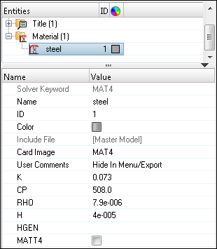
Figure 3.Since you are conducting a purely heat transfer analysis, structural isotropic properties (for example, MAT1 card) are not required. Also, it is assumed that the thermal material properties (MAT4) are temperature independent.
A new material, steel, is created with thermal properties necessary for a transient heat transfer analysis.
Now, create the solid property for this model referencing the PSOLID entry and connect the material, steel, to this property; the property can then be assigned to the existing component.
-
In the Select Material dialog, select
steel and click OK.
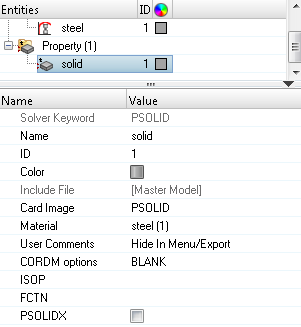
Figure 4.
Link Thermal Material and Property to the Structure
-
In the Select Property
dialog, select solid and
click OK.
The material steel now is automatically linked to the component auto1.
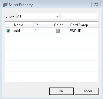
Figure 5.
Create Transient Heat Transfer Analysis Time Steps
-
Click
 and enter the number of time steps (N) = 50 and set each
time increment (DT) to 10.
This encompasses a total time period of 500 seconds in which to capture the behavior of the system.
and enter the number of time steps (N) = 50 and set each
time increment (DT) to 10.
This encompasses a total time period of 500 seconds in which to capture the behavior of the system.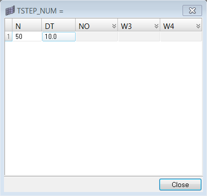
Figure 6.
Create Transient Heat Transfer Analysis Initial Conditions
-
For T1, enter a value of
25.

Figure 7.
Apply Ambient Temperature Boundary Conditions
Ambient temperature thermal boundary conditions is applied on the model by creating specific load collectors for each. The ambient temperature is controlled using an SPCD entry, as this will allow an ambient temperature variation over time to help mimic such physical requirements (if any).
Create a Time-variant Ambient Temperature
-
If the Ambient SPCD load collector is not specified, right-click
Ambient SPCD in the Model Browser
and click Make Current.
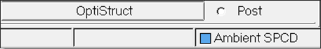
Figure 8. Displaying the Current Load Collector - Ambient SPCD -
For load types =, select SPCD.
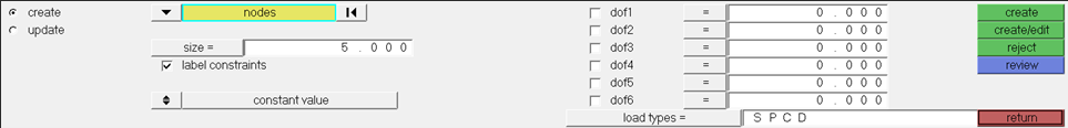
Figure 9. Creating an SPCD Entry to Control the Ambient Temperature
Checkpoint
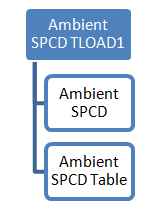
Figure 10. Process to specify a time-variant SPCD
-
For load types =, select SPC.
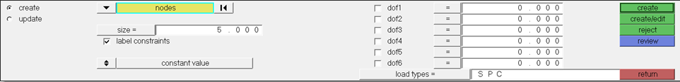
Figure 11. Creating the SPC Boundary Condition
Apply Heat Flux Load
Ambient temperature thermal boundary conditions have been assigned to the model and heat flux load from the outer surface of the engine (to which the fin is attached) is applied on the model. A time-varying heat flux load of 0 to 0.1 W/mm2 from 0 to 500 seconds is used for the analysis of this fin. This load is applied on the model by creating specific load collectors for the corresponding TLOAD1, QBDY1 and TABLED1 entries similar to the procedure used for the ambient temperature SPCD definition.
Create a Time-variant Linearly Increasing Heat Flux Load
-
If the Heat Flux QBDY1 load collector is not
specified, right-click Heat Flux
QBDY1 in the Entity Editor and click
Make Current.
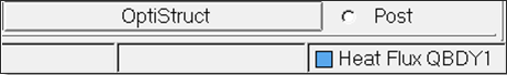
Figure 12. Display the Current Load Collector - Heat Flux QBDY1 -
Check the box next to Element_set_Flux and
click select.
The predefined element set is now highlighted in white on the model.
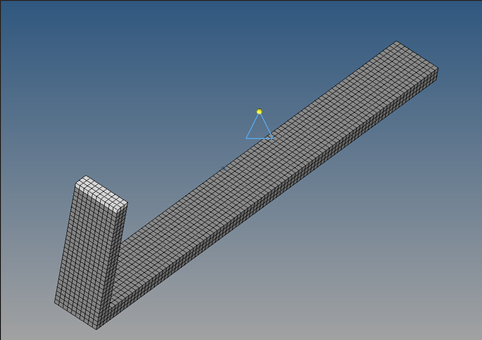
Figure 13. Highlighted Element Set is Displayed in WhiteTip: The break angle helps find adjacent solid faces for the same element set; however, since this surface element set generation requires only one face, the value of the break angle is not germane in this situation. -
Click nodes and select
the nodes in the Figure 14.
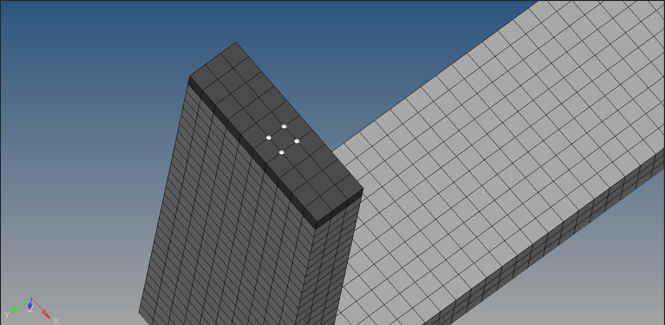
Figure 14. Select the Nodes on the Highlighted Surface for Conduction Surface Element Creation -
Click Close.
A conduction interface is created because QBDY1 data can only reference surface elements and the conduction interface helps us create a set of surface elements at the surface where heat flux is input.
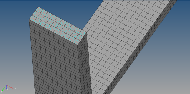 Figure 15. Newly Generated Surface Elements are Displayed in Blue
 -
Next, create the amplitude (constant part) of the time variant heat flux using a
QBDY1 Data Entry. Do this by clicking on .
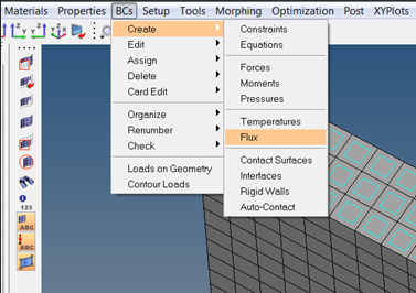
Figure 16. Access the Flux Creation Panel -
Enter 0.1 in the value=
field and select QBDY1 in
the load types = field. Specify any low value in
the magnitude% =field to assign a value to the
size of the display label for the flux load.
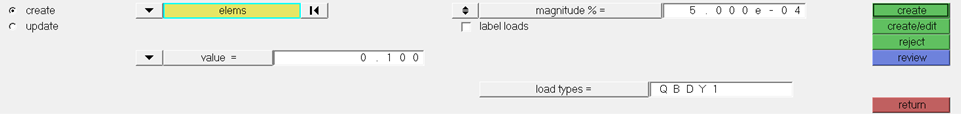
Figure 17. Heat Flux Load Panel -
Click next to Data. In the pop-out
window, enter x(1) =
0.0,y(1) =
0.0, x(2) =
500.0 and y(2) =
1.0.
Tip: In this tutorial, a linearly incremental heat flux load (the values of y(1) and y(2) are 0 and 1 leading to a linearly increasing heat flux distribution over the first 500 seconds) is defined.
Checkpoint
The QBDY1 flux load and its corresponding table are linked to the previously created TLOAD1 entry.
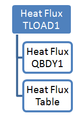
Figure 18. Process to Specify a Time-Variant SPCD
Add Free Convection
Free convection is assigned in a similar manner to the procedure used for the creation of the conduction interface. Free convection is, however, automatically assigned to all heat transfer subcases and the PCONV and CONV entries should refer to the material, steel, and the ambient temperature. The ambient temperature calculates the amount of heat transferred through free convection.
Create Surface Elements for Free Convection
-
Select element set
Element_set_Convection and
click select. The
predefined element set is now highlighted in white
on the model.
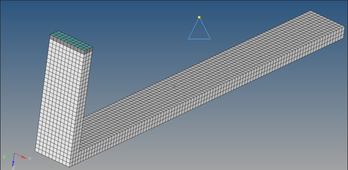
Figure 19. Highlighted Element Set is Displayed in White -
Click the MID field and
select steel from the
menu.
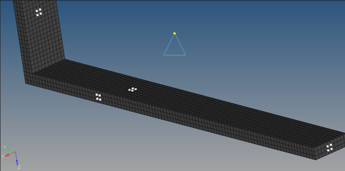
Figure 20. Select the Nodes on Four of the Seven Highlighted Surfaces for Convection Surface Element Creation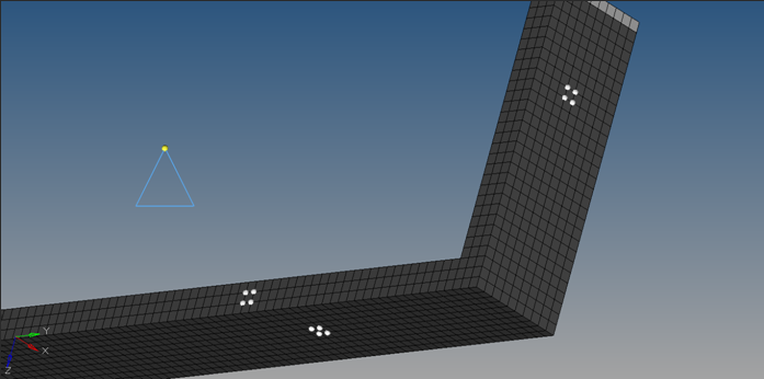
Figure 21. Select Nodes on the Three Remaining Highlighted Surfaces for the Creation of a Convection InterfaceThe newly created CHBDYE surface elements are displayed in yellow, as shown in Figure 22 below.
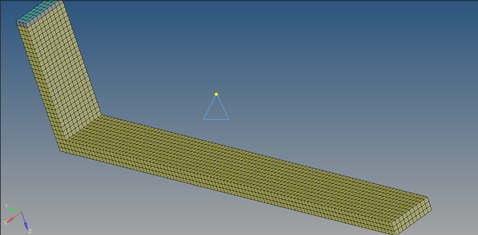
Figure 22. Newly Generated CHBBDYE Surface Elements are Displayed in Yellow on the ModelA new group convection_interface is created in the Model Browser. -
Next, the convection boundary condition is defined by referencing the ambient
temperature in the CONV Data Entry. This is done by clicking on the
Card Edit icon
 and selecting the elems entry.
Combine TLOAD1 Entries into a DLOAD Entry
-
Click
next to Data below the DLOAD_NUM field. In the DLOAD_NUM pop-up window, enter
S(1) = 1.0 and S(2) = 1.0.
-
Click Close.
Checkpoint
The DLOAD entry is created as a linear combination of two TLOAD1 entries - Heat Flux TLOAD1 and Ambient SPCD TLOAD1.
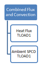
Figure 23. Process to Specify a Time-variant SPCD
Create a Transient Heat Transfer Load Step
Submit the Job
-
From the Analysis page, click the OptiStruct
panel.
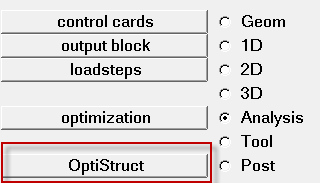
Figure 24. Accessing the OptiStruct Panel
View Results
-
On the Results toolbar, click
 to open the
Contour panel.
to open the
Contour panel.
-
Select the first pull-down menu below Result type and select Grid
Temperatures(s).
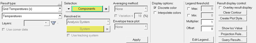
Figure 25. Contour Plot Panel in HyperView -
Click Apply, select Time =
5.0000000E+02 from the Results Browser.
A contour plot of grid temperatures at the final time step is created as shown in Figure 26.
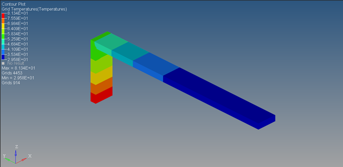
Figure 26. Grid Temperature Contour for the Final Time Step (500 seconds) - WITH FREE CONVECTION
Checkpoint
In Figure 26, this is the grid point temperature plot after 500 seconds. The system is input a linearly increasing heat flux from 0 to 0.1 W/mm2 from 0 to 500 seconds respectively. Therefore, a physical correlation can be the effect of starting an IC engine to full capacity wherein the flux transmitted to the outer surface linearly increases with time. Note that the flux patterns in actuality may be different and may fluctuate based on the duration of the power cycles. The maximum temperature of 81.3°C predictably occurs at the elements closest to the heat flux loading site and the minimum temperature of 29.5°C occurs at elements farthest from the heat source.
-
Click Apply, select Time =
2.0000000E+01 from the Results Browser.
A contour plot of grid temperatures is created, as shown in Figure 27.
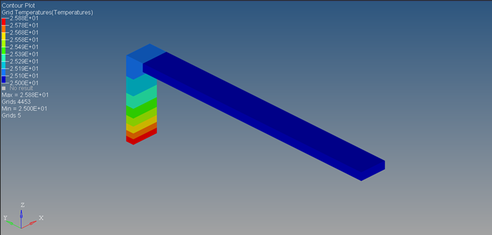
Figure 27. Grid Temperature Contour Plot after 20 Seconds - WITH FREE CONVECTION
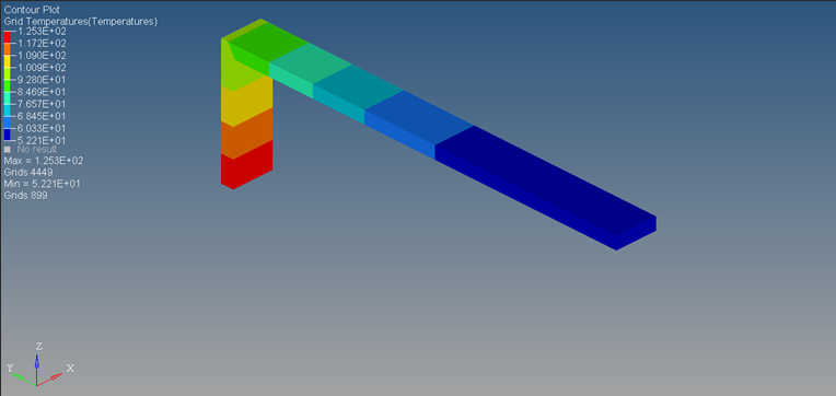
Figure 28. Grid Temperature Contour Plot after 500 Seconds - WITHOUT FREE CONVECTION
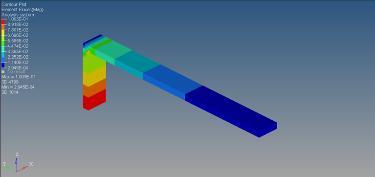
Figure 29. Contour Plot of Element Fluxes after 500 Seconds