OS-T: 1020 Normal Modes Analysis of a Splash Shield

In this tutorial, an existing finite element model of an automotive splash shield is used to demonstrate how to set up and perform a normal modes analysis. HyperView post-processing tools are used to determine mode shapes of the model.

The sshield.fem file is needed to perform this tutorial.

Launch HyperMesh and Set the OptiStruct User Profile

  1. Launch HyperMesh.
    The User Profile dialog opens.
  2. Select OptiStruct and click OK.
    This loads the user profile. It includes the appropriate template, macro menu, and import reader, paring down the functionality of HyperMesh to what is relevant for generating models for OptiStruct.

Import the Model

  1. Click File > Import > Solver Deck.
    An Import tab is added to your tab menu.
  2. For the File type, select OptiStruct.
  3. Select the Files icon files_panel.
    A Select OptiStruct file browser opens.
  4. Select the sshield.fem file you saved to your working directory. Refer to Access the Model Files.
  5. Click Open.
  6. Click Import, then click Close to close the Import tab.

Set Up the Model

Review Properties of Rigid Elements

There are two rigid "spiders" in the model that are placed at locations where the shield is bolted down. This is a simplified representation of the interaction between the bolts and the shield. It is assumed that the bolts are significantly more rigid in comparison to the shield.

To be able to distinguish the spiders clearly in the model, you will use the Shaded Elements and Mesh Lines icon visualizationElementsShadedWithMesh-24.

The dependent nodes of the rigid elements have all six degrees of freedom constrained. Therefore, each "spider" connects nodes of the shell mesh together in such a way that they do not move with respect to one another. Revert to the Wireframe Elements Skin Only mode by clicking on the visualizationElementsWireframeSkinOnly-24 icon.

  1. From the menu bar, click Mesh > Edit > 1D Elements > Rigids to open the Rigids panel.
  2. Click review.
  3. Select one of the rigid elements.
    In the modeling window, HyperMesh displays the IDs of the rigid element and the two end nodes and indicates the independent node with an 'I' and the dependent node with a 'D'. HyperMesh also indicates the constrained degrees of freedom for the selected element, through the dof check boxes in the Rigids panel. All rigid elements in this model should have all DOFs constrained.
  4. Click return to go back to the main menu.

Create the Material

The imported model has four component collectors with no materials. A material collector needs to be created and assigned to the shell component collectors. The rigid elements do not need to be assigned a material.

  1. In the Model Browser, right-click and select Create > Material from the context menu.
    A default material displays in the Entity Editor.
  2. For Name, enter steel.
  3. Set Card Image to MAT1.
  4. Enter the material values next to the corresponding fields.
    1. For E (Young's Modulus), enter 2E+05.
    2. For NU, (Poisson's Ratio), enter 0.3.
    3. For RHO (Mass Density), enter 7.85E-009.
      A material density is required for the normal modes solution sequence.


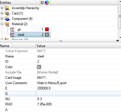
    Figure 1. Material Property Values for steel
A new material, steel, has been created. The material uses OptiStruct's linear isotropic material model, MAT1.

Edit the Properties

Shell thickness values also need to be corrected.
  1. In the Model Browser, Properties folder, click design.
    The design property entry is displayed in the Entity Editor.
  2. For T (thickness), enter 0.25.
  3. Change the material assigned to the property from gn to steel.
    1. For Material, click (1) gn > Material.
    2. In the Select Material dialog, select steel and click OK.
  4. Similarly, on the property nondesign, update T (thickness) to 0.25 and change the material from gn to steel.

OS_1010_07
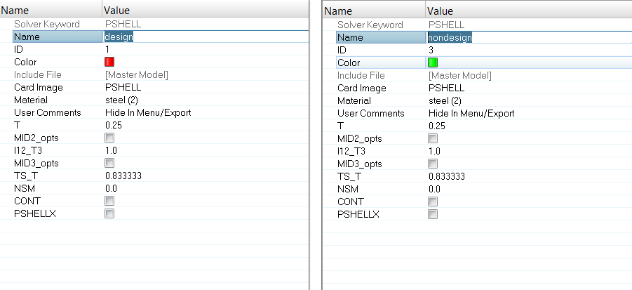
Figure 2. Updating the Thickness Value for Design and Nondesign Property Entries

Apply Loads and Boundary Conditions

The model is to be constrained using SPCs at the bolt locations. The constraints are organized into the load collector 'constraints'.

To perform a Normal Modes Analysis, a real eigenvalue extraction (EIGRL) card needs to be referenced in the subcase. The real eigenvalue extraction card is defined in HyperMesh as a load collector with an EIGRL card image. This load collector should not contain any other loads.

Create EIGRL Card

In the following steps, the model is constrained so that two opposing edges of the four external edges cannot move. The other two edges remain unconstrained. A total load of 1000N is applied at the edge of the hole in the positive z-direction.
  1. In the Model Browser, right-click and select Create > Load Collector from the context menu.
    A default load collector displays in the Entity Editor.
  2. For Name, enter EIGRL.
  3. For Card Image, select EIGRL.

    OS_1010_08
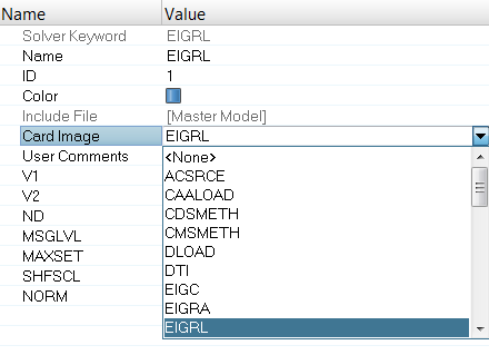
    Figure 3. Select the Card Image
  4. Click Color and select a color from the color palette.
  5. For V2, enter 200.000.
  6. For ND, enter 6.

    OS_1010_09
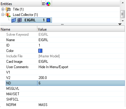
    Figure 4. Create New Load Collector "EIGRL" in the Model Browser

Create Constraints

  1. Create a load collector, named constraints.
  2. From the menu bar, click BCs > Create > Constraints to open the Constraints panel.
  3. With the nodes selector active, select the two nodes at the center of the rigid spiders.

    rd1020_constraints
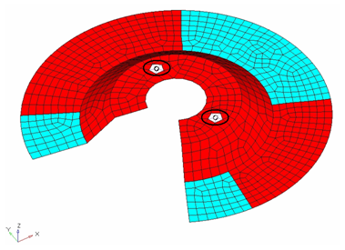
    Figure 5. Select Nodes for Constraining the Bolt Locations
  4. Constrain all DOFs with a value of 0.0.
  5. Set load types= to SPC.
  6. Click create.
    Two constraints are created. Constraint symbols (triangles) appear in the modeling window at the selected nodes. The number 123456 is written beside the constraint symbol, if the label constraints is checked "ON", indicating that all DOFs are constrained.
  7. Click return.

Create Load Steps

  1. In the Model Browser, right-click and select Create > Load Step from the context menu.
    A default load step displays in the Entity Editor.
  2. For Name, enter bolted.
  3. Set Analysis type to Normal modes.
  4. Define SPC.
    1. For SPC, click Unspecified > Loadcol.
    2. In the Select Loadcol dialog, select constraints and click OK.
  5. Define METHOD(STRUCT).
    1. For METHOD(STRUCT), click Unspecified > Loadcol.
    2. In the Select Loadcol dialog, select EIGRL and click OK.

An OptiStruct subcase has been created which references the constraints in the load collector constraints and the real eigenvalue extraction data in the load collector EIGRL.


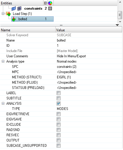
Figure 6. Creating the bolted Loadstep

Submit the Job

  1. From the Analysis page, click the OptiStruct panel.

    OS_1000_13_17
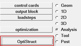
    Figure 7. Accessing the OptiStruct Panel
  2. Click save as.
  3. In the Save As dialog, specify location to write the OptiStruct model file and enter sshield_complete for filename.
    For OptiStruct input decks, .fem is the recommended extension.
  4. Click Save.
    The input file field displays the filename and location specified in the Save As dialog.
  5. Set the export options toggle to all.
  6. Set the run options toggle to analysis.
  7. Set the memory options toggle to memory default.
  8. Click OptiStruct to launch the OptiStruct job.
If the job is successful, new results files should be in the directory where the sshield_complete.fem was written. The sshield_complete.out file is a good place to look for error messages that could help debug the input deck if any errors are present.
The default files written to the directory are:
sshield_complete.html
HTML report of the analysis, providing a summary of the problem formulation and the analysis results.
sshield_complete.out
OptiStruct output file containing specific information on the file setup, the setup of your optimization problem, estimates for the amount of RAM and disk space required for the run, information for each of the optimization iterations, and compute time information. Review this file for warnings and errors.
sshield_complete.h3d
HyperView binary results file.
sshield_complete.res
HyperMesh binary results file.
sshield_complete.stat
Summary, providing CPU information for each step during analysis process.

View the Results

Eigenvector results are output by default, from OptiStruct for a Normal Modes Analysis. This section describes how to view the results in HyperView.

Load the Model and Result Files

In this step, you will load a file into the HyperView animation window.
  1. When the message ANALYSIS COMPLETED is received in the Mechanical Solver View window, click Results.
    HyperView is launched and the results are loaded.
  2. Click Close to close the message window, if one appears.

View the Deformed Shape

It is helpful to view the deformed shape of a model to determine if the boundary conditions have been defined correctly and also to check if the model is deforming as expected. In this section, use the Deformed panel to review the deformed shape for last mode.
  1. Click the animation selector switch in the lower toolbar animationLinear-24 and select Set Modal Animation Mode animationModal-24 .
  2. Select the Deformed toolbar icon resultsDeformed-24.
  3. Leave Result type set to Eigen mode (v).
  4. Set Scale to Model units.
  5. Set Type to Uniform and enter in a scale factor of 10 for Value.
    • This means that the maximum displacement will be 10 modal units and all other displacements will be proportional.
    • Use a scale factor higher than 1.0 to amplify the deformations while a scale factor smaller than 1.0 would reduce them. In this case, displacements are accentuated in all directions.

    OS_1010_11
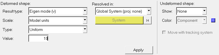
    Figure 8. Deformed Shape Panel
  6. Click Apply.
  7. Under Undeformed shape, set Show to Wireframe.
    A deformed plot of the model overlaid on the original undeformed mesh is displayed in the modeling window.
  8. In the Results Browser pull-down menu, you can change the view between various subcases using the Load Case and Simulation Selection drop-down menus, as shown below:
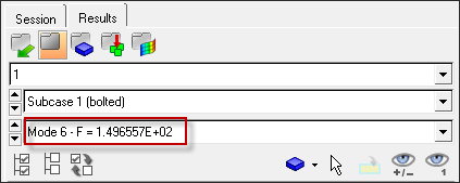
    rd1020_hv_results
    Figure 9.
  9. Select Mode 6 - F=1.496557E+02 from the list to view Mode 6.
  10. To animate the mode shape, click Start/Pause Animation animationStart-24 in the Animation toolbar.
  11. To control the animation speed, use the Animation Controls on the Animation toolbar, as shown below:
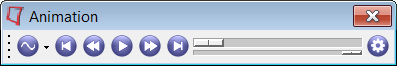
    animation_toolbar
    Figure 10.
  12. Review the other mode shapes.

Summary

In this analysis, it was assumed that the bolts were significantly stiffer than the shield. If the bolts needed to be made of aluminum and the shield was still made of steel, would the model need to be modified, and the analysis run again?

It is necessary to push the natural frequencies of the splash shield above 50 Hz. With the current model, there should be one mode that violates this constraint: Mode 1. Design specifications allow the inner disjointed circular rib to be modified such that no significant mass is added to the part. Is there a configuration for this rib within the above stated constraints that will push the first mode above 50 Hz? See tutorial OS-T: 2020 Increase Natural Frequencies of an Automotive Splash Shield with Ribs to optimize rib locations for this part.