OS-T: 2020 Increase Natural Frequencies of an Automotive Splash Shield with Ribs

In this tutorial you will generate a preliminary design of stiffeners in the form of ribs for an automotive splash shield. The objective is to increase the natural frequency of the first normal mode using topology to identify locations for ribs in the designable region.


os2020_pic1
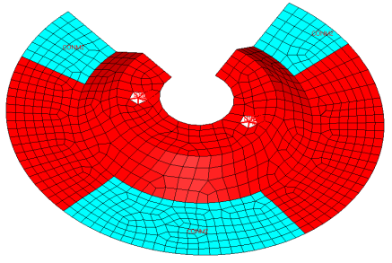
Figure 1. Finite Element Mesh. The finite element mesh contains designable (red) and non-designable (blue) material.
The optimization problem for this tutorial is stated as:
Objective
Maximize frequency of mode number 1.
Constraint
Upper bound constraint of 40% for the designable volume.
Design Variables
Density of each element in the design space.

Launch HyperMesh and Set the OptiStruct User Profile

  1. Launch HyperMesh.
    The User Profile dialog opens.
  2. Select OptiStruct and click OK.
    This loads the user profile. It includes the appropriate template, macro menu, and import reader, paring down the functionality of HyperMesh to what is relevant for generating models for OptiStruct.

Import the Model

  1. Click File > Import > Solver Deck.
    An Import tab is added to your tab menu.
  2. For the File type, select OptiStruct.
  3. Select the Files icon files_panel.
    A Select OptiStruct file browser opens.
  4. Select the sshield_opti.fem file you saved to your working directory. Refer to Access the Model Files.
  5. Click Open.
  6. Click Import, then click Close to close the Import tab.

Apply Loads and Boundary Conditions

Create Load Collectors

  1. Create the Constraints load collector.
    1. In the Model Browser, right-click and select Create > Load Collector from the context menu.
      A default load collector displays in the Entity Editor.
    2. For Name, enter constraints.
    3. Click Color and select a color from the color palette.
    4. Set Card Image to None.
  2. Create the EIGRL load collector.
    1. In the Model Browser, right-click and select Create > Load Collector from the context menu.
      A default load collector displays in the Entity Editor.
    2. For Name, enter EIGRL.
    3. Click Color and select a color from the color palette.
    4. Set Card Image to EIGRL.
    5. For V2, enter 3000.
    6. For ND, enter 2.
    This load collector defines data needed to perform real eigenvalue analysis (vibration or buckling) and specified the solver to calculate the first two modes between a frequency range of 0 and 3000 Hz.

Create Constraints

In this step you will create constraints at bolt locations.
  1. From the Model Browser, Load Collectors folder, right-click on Constraints and select Make Current from the context menu.
  2. From the Analysis page, click constraints.
  3. Select the Create subpanel.
  4. Double-click nodes and select by id, then enter 1075, 1076 in the id= field.
  5. Constrain all dofs.
    Dofs with a check will be constrained, while dofs without a check will be free. Dofs 1, 2, and 3 are x, y, and z translation degrees of freedom. Dofs 4, 5, and 6 are x, y, and z rotational degrees of freedom.
  6. Click create.
  7. Click return to go to the main menu.
Two constraints are now created. Constraint symbols (triangles) appear at the selected nodes. The number 123456 is displayed beside the constraint symbol, indicating that all dofs are constrained.

Create Load Steps

  1. In the Model Browser, right-click and select Create > Load Step from the context menu.
    A default load step displays in the Entity Editor.
  2. For Name, enter frequencies.
  3. Set Analysis type to normal modes.
  4. Define SPC.
    1. For SPC, click Unspecified > Loadcol.
    2. In the Select Loadcol dialog, select constraints and click OK.
  5. Define METHOD(STRUCT).
    1. For METHOD(STRUCT), click Unspecified > Loadcol.
    2. In the Select Loadcol dialog, select EIGRL and click OK.

Submit the Job

  1. From the Analysis page, click the OptiStruct panel.

    OS_1000_13_17
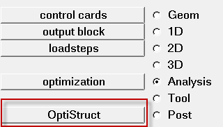
    Figure 2. Accessing the OptiStruct Panel
  2. Click save as.
  3. In the Save As dialog, specify location to write the OptiStruct model file and enter sshield_analysis for filename.
    For OptiStruct input decks, .fem is the recommended extension.
  4. Click Save.
    The input file field displays the filename and location specified in the Save As dialog.
  5. Set the export options toggle to all.
  6. Set the run options toggle to analysis.
  7. Set the memory options toggle to memory default.
  8. Clear the options field.
  9. Click OptiStruct to launch the OptiStruct job.
If the job is successful, new results files should be in the directory where the sshield_analysis.fem was written. The sshield_analysis.out file is a good place to look for error messages that could help debug the input deck if any errors are present.
The default files written to the directory are:
sshield_analysis.html
HTML report of the analysis, providing a summary of the problem formulation and the analysis results.
sshield_analysis.out
OptiStruct output file containing specific information on the file setup, the setup of your optimization problem, estimates for the amount of RAM and disk space required for the run, information for each of the optimization iterations, and compute time information. Review this file for warnings and errors.
sshield_analysis.h3d
HyperView binary results file.
sshield_analysis.res
HyperMesh binary results file.
sshield_analysis.stat
Summary, providing CPU information for each step during analysis process.
sshield_analysis.mvw
HyperView session file.
sshield_analysis_frames.html
HTML file used to post-process the .h3d with HyperView Player using a browser. It is linked with the _menu.html file.
sshield_analysis_menu.html
HTML file to post-process the .h3d with HyperView Player using a browser.

View the Results

Eigenvector results are output from OptiStruct for a normal modes analysis by default. This section describes how to view the results in HyperView.
  1. From the OptiStruct panel, click HyperView.
    HyperView launches inside of page 2 of HyperMesh Desktop, and displays the sshield_analysis.mvw session file, which is linked with the sshield_analysis.h3d file.
  2. From the Animation toolbar, set the animation mode to animationModal-24 (Modal).
  3. In the Results browser, click Mode 1.
    The browser shows the first two natural frequencies calculated between 0 and 3000Hz.
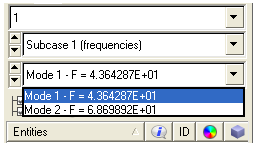
    os_2020_mode_shapes
    Figure 3.
  4. Define deformed settings.
    1. From the Results toolbar, click resultsDeformed-24 to open the Deformed panel.
    2. Set Result type to Eigen mode (v).
    3. Set Scale to Model Units.
    4. Set Type to Uniform.
    5. In the Value field, enter 10.
    6. Click Apply.
  5. Animate the model.
    1. From the Animation toolbar, click animationOptions-24.
    2. Move the Max Frame Rate slider between 60 and 1 to increase or decrease the animation speed.
      Tip: You can also change the default values for Angular Increment to refine your animation.
    3. Click animationStart-24 to start the animation.
      An animation of the mode shape should be seen for the first frequency.
    4. Click to stop the animation.
  6. On the Page Control toolbar, click the Page Delete icon to delete the HyperView page.
    page_delete Figure 4.

Set Up the Optimization

Create Topology Design Variables

  1. From the Analysis page, click optimization.
  2. Click topology.
  3. Select the create subpanel.
  4. In the desvar= field, enter shield.
  5. Set type: to PSHELL.
  6. Using the props selector, select design.
  7. For base thickness, enter 0.300.
  8. Click create.

    A topology design space definition, shield, has been created. All elements referring to the design property collector (elements organized into the "design" component collector) are now included in the topology design space. The thickness of these shells can vary between 0.300 (base thickness) and the maximum thickness defined by the T (thickness) field on the PSHELL card.

    The object of this exercise is to determine where to locate ribs in the designable region. Therefore, a non-zero base thickness is defined, which is the original thickness of the shells. The maximum thickness, which is defined by the T field on the PSHELL card, should be the allowable depth of the rib.

    Currently, the T field on the PSHELL card is still set to 0.300 (the original shell thickness). You will change this to 1.0 so that the ribs of a maximum height of 0.7 units can be obtained by the topology optimization.

  9. Click return.
  10. Edit the thickness of the design property.
    1. In the Model Browser, Properties folder, click design.
    2. In the Entity Editor, T field, enter 1.000.

Create Optimization Responses

  1. From the Analysis page, click optimization.
  2. Click Responses.
  3. Create the volume fraction response.
    1. In the responses= field, enter volfrac.
    2. Below response type, select volumefrac.
    3. Set regional selection to total and no regionid.
    4. Click create.
  4. Create the frequency response.
    1. In the responses= field, enter freq1.
    2. Below response type, select frequency.
    3. For Mode Number, enter 1.0.
    4. Click create.
    A response, freq1, is defined for the frequency of the first mode extracted.
  5. Click return to go back to the Optimization panel.

Define the Objective Function

  1. Click the objective panel.
  2. Verify that max is selected.
  3. Click response= and select freq1.
  4. Using the loadsteps selector, select frequencies.
  5. Click create.
  6. Click return twice to exit the Optimization panel.

Define Constraints

A response defined as the objective cannot be constrained. In this case, you cannot constrain the response freq1. An upper bound constraint needs to be defined for the response volfrac.

  1. Click dconstraints.
  2. In the constraint= field, enter volume_constr.
  3. Check the box next to upper bound, then enter 0.40.
  4. Click response = and select volfrac.
  5. Click create.
  6. Click return to return to the Optimization panel.
A constraint is defined on the response volfrac. The constraint is an upper bound with a value of 0.40. The constraint applies to all subcases as the volumefrac response is a global response. In this step you are allowing the topology optimization to use additional volume with which it can come with ribsvconstr.

Run the Optimization

  1. From the Analysis page, click OptiStruct.
  2. Click save as.
  3. In the Save As dialog, specify location to write the OptiStruct model file and enter sshield_optimization for filename.
    For OptiStruct input decks, .fem is the recommended extension.
  4. Click Save.
    The input file field displays the filename and location specified in the Save As dialog.
  5. Set the export options toggle to all.
  6. Set the run options toggle to optimization.
  7. Set the memory options toggle to memory default.
  8. Click OptiStruct to run the optimization.
    The following message appears in the window at the completion of the job:
    OPTIMIZATION HAS CONVERGED.
    FEASIBLE DESIGN (ALL CONSTRAINTS SATISFIED).
    OptiStruct also reports error messages if any exist. The file sshield_optimization.out can be opened in a text editor to find details regarding any errors. This file is written to the same directory as the .fem file.
  9. Click Close.
The default files that get written to your run directory include:
sshield_optimization.mvw
HyperView session file.
sshield_optimization.HM.comp.cmf
HyperMesh command file used to organize elements into components based on their density result values. This file is only used with OptiStruct topology optimization runs.
sshield_optimization.out
OptiStruct output file containing specific information on the file setup, the setup of the optimization problem, estimates for the amount of RAM and disk space required for the run, information for all optimization iterations, and compute time information. Review this file for warnings and errors that are flagged from processing the sshield_optimization.fem file.
sshield_optimization.sh
Shape file for the final iteration. It contains the material density, void size parameters and void orientation angle for each element in the analysis. This file may be used to restart a run.
sshield_optimization.hgdata
HyperGraph file containing data for the objective function, percent constraint violations, and constraint for each iteration.
sshield_optimization.oss
OSSmooth file with a default density threshold of 0.3. You may edit the parameters in the file to obtain the desired results.
sshield_optimization.stat
Contains information about the CPU time used for the complete run and also the break-up of the CPU time for reading the input deck, assembly, analysis, convergence, and so on.
sshield_optimization.his_data
The OptiStruct history file containing iteration number, objective function values and percent of constraint violation for each iteration.
sshield_optimization.HM.ent.cmf
HyperMesh command file used to organize elements into entity sets based on their density result values. This file is only used with OptiStruct topology optimization runs.
sshield_optimization.html
HTML report of the optimization, giving a summary of the problem formulation and the results from the final iteration.
sshield_optimization_frame.html
HTML file used to post-process the .h3d with HyperView Player using a browser. It is linked with the _menu.html file.
sshield_optimization_menu.html
HTML file used to post-process the .h3d with HyperView Player using a browser.
sshield_optimization_des.H3D
HyperView binary results file that contains: Density results from topology optimizations, Shape results from topography or shape optimizations and Thickness results from size and topology optimizations.
sshield_optimization_s1.H3D
HyperView binary results file that contains: Displacement results from linear static analysis, Element strain energy results from normal mode analysis and Stress results from linear static analysis, etc.

View the Results

With topology optimization of shell elements, Element Density and Element Thickness results are output from OptiStruct for all iterations. In addition, Eigenvector results are output for the first and last iterations by default. This section describes how to view those results in HyperView.
  1. From the OptiStruct panel, click HyperView.

    HyperView launches inside of HyperMesh Desktop, and loads the session file sshield_optimization.mvw that is linked with the sshield_optimization_des.h3d and the sshield_optimization_s1.h3d.

  2. From the Results toolbar, click resultsContour-24 to open the Contour panel.
  3. Set the Result type: to Element Densities(s).
  4. Click Apply.
  5. From the Results Browser, select the last iteration.
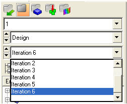
    os_2020_iteration
    Figure 5.

    Each element of the model is assigned a legend color, indicating the density of each element for the selected iteration.

    Analyze the following:
    Have most of your elements converged to a density close to 1 or 0?
    If there are many elements with intermediate densities, the discrete parameter may need to be adjusted. The DISCRETE parameter (set in the Opti control panel on the Optimization panel) can be used to push elements with intermediate densities towards 1 or 0 so that a more discrete structure is given.
    Regions that need reinforcement tend towards a density of 1.0. Areas that do not need reinforcement tend towards a density of 0.0.
    Is the max = field showing 1.0e+00?
    In this case, it is.
    If it is not, the optimization has not progressed far enough. Allow more iterations and/or decrease the OBJTOL parameter (set in the Opti control panel).
    If adjusting the DISCRETE parameter, incorporating a checkerboard control, refining the mesh, and/or decreasing the objective tolerance does not yield a more discrete solution (none of the elements progress to a density value of 1.0), you may want to review the set up of the optimization problem. Some of the defined constraints may not be attainable for the given objective function (or visa-versa).

    os_2020_contour
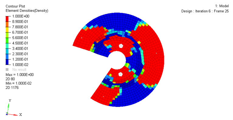
    Figure 6. Contour Plot of Element Densities at iteration 6 (top view)
    Where would you place your ribs?
  6. On the Page Control toolbar, click the Page Delete icon to delete the HyperView page.

    page_delete
    Figure 7.

Set Up the Final Normal Modes Analysis

Based on the topology results obtained above, a number of ribs were added to the model. The new design sshield_newdesign.fem, which includes these ribs can be found in the optistruct.zip file.

Delete the Current Model

  1. In HyperMesh, click return to exit the OptiStruct panel.
  2. From the menu bar, click File > New > Model.
  3. Click Yes to clear the current session.
    Deleting the current model clears the current HyperMesh database. Information stored in .hm files on your disk is not affected.

Import the Model

  1. Click File > Import > Solver Deck.
    An Import tab is added to your tab menu.
  2. For the File type, select OptiStruct.
  3. Select the Files icon files_panel.
    A Select OptiStruct file browser opens.
  4. Select the sshield_newdesign.fem file you saved to your working directory. Refer to Access the Model Files.
  5. Click Open.
  6. Click Import, then click Close to close the Import tab.

Submit the Job

  1. From the Analysis page, click the OptiStruct panel.

    OS_1000_13_17
    Figure 8. Accessing the OptiStruct Panel
  2. Click save as.
  3. In the Save As dialog, specify location to write the OptiStruct model file and enter sshield_newdesign for filename.
    For OptiStruct input decks, .fem is the recommended extension.
  4. Click Save.
    The input file field displays the filename and location specified in the Save As dialog.
  5. Set the export options toggle to all.
  6. Set the run options toggle to analysis.
  7. Set the memory options toggle to memory default.
  8. Clear the options field.
  9. Click OptiStruct to launch the OptiStruct job.
If the job is successful, new results files should be in the directory where the sshield_newdesign.fem was written. The sshield_newdesign.out file is a good place to look for error messages that could help debug the input deck if any errors are present.
The default files written to the directory are:
sshield_newdesign.html
HTML report of the analysis, providing a summary of the problem formulation and the analysis results.
sshield_newdesign.out
OptiStruct output file containing specific information on the file setup, the setup of your optimization problem, estimates for the amount of RAM and disk space required for the run, information for each of the optimization iterations, and compute time information. Review this file for warnings and errors.
sshield_newdesign.h3d
HyperView binary results file.
sshield_newdesign.res
HyperMesh binary results file.
sshield_newdesign.stat
Summary, providing CPU information for each step during analysis process.
sshield_newdesign.mvw
HyperView session file.
sshield_newdesign_frames.html
HTML file used to post-process the .h3d with HyperView Player using a browser. It is linked with the _menu.html file.
sshield_newdesign_menu.html
HTML file to post-process the .h3d with HyperView Player using a browser.

View the Results

  1. From the OptiStruct panel, click HyperView.
    This launches HyperView in the HyperMesh Desktop and loads the file sshield_newdesign.mvw that is linked with the file sshield_newdesign.h3d.
  2. Set the animation mode to animationModal-24 (Modal).
  3. In the Results Browser, select Mode 1.
  4. Click resultsDeformed-24 to open the Defomed panel.
  5. Make or verify the following settings in the Deformed panel.
    Result Type
    Eigen mode (v)
    Scale
    Model Units
    Type
    Uniform
    Value
    10
  6. Click Apply.
  7. Click animationStart-24 to start the animation.
    An animation of the mode shape should be seen for the first frequency.
  8. Click animationStart-24 again to stop the animation.

Compare Results

What is the percentage increase in frequency for your first mode (sshield_analysis.fem versus sshield_newdesign)?

You have seen that the frequency of the structure for the first mode has increased from 43.63 Hz to 84.88 Hz.

How much mass has been added to the part (check the mass of your ribs in the mass calc panel in the Tool page)?

What is the percentage increase in mass?