OS-T: 2030 Control Arm with Draw Direction Constraints
In this tutorial you will perform a topology optimization using draw direction
constraints on a control arm.
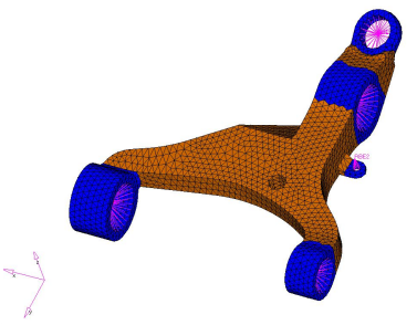
The finite element mesh contains designable (brown) and non-designable regions (blue)
is shown in Figure 1. Figure 1. Control Arm Schematic
Launch HyperMesh and Set the OptiStruct User Profile
Launch HyperMesh.
The User Profile dialog opens.
Select OptiStruct and click
OK.
This loads the user profile. It includes the appropriate template, macro
menu, and import reader, paring down the functionality of HyperMesh to what is relevant for generating models for
OptiStruct.
Open the Model
Click File > Open > Model.
Select the controlarm.hm file you saved to
your working directory from the optistruct.zip file. Refer
to Access the Model Files.
Click Open.
The controlarm.hm database is loaded
into the current HyperMesh session, replacing any
existing data.
Set Up the Optimization
Create Topology Design Variables
From the Analysis page, click optimization.
Click topology.
Select the create subpanel.
In the desvar= field, enter dv1.
Set type: to PSOLID.
Using the props selector, select Design.
Click create.
Create Draw Direction Constraints
The draw direction constraints allow the casting feasibility of the design so that the
topology determined will allow the die to slide in a given direction. These constraints
are defined using the DTPL card. Two DRAW options are available. The
option 'SINGLE' assumes that a single die will be used. The option
'SPLIT' assumes that two dies splitting apart in the given draw
direction will be used to cast the part.
Select the draw subpanel.
Set draw type: to single.
The option 'SINGLE' assumes that a single die will be used
and it slides in the given drawing direction.
Define the drawing direction.
Click anchor node, and enter
3209 in the id= field.
Click first node, and enter
4716 in the id= field.
Using the props selector, select the Non-design
property.
The non-designable parts are selected as obstacles for the casting
process on the same DTPL card, and the casting feasibility of
the final structure is persevered.
Click update.
Click return to go back to the Optimization panel.
Create Optimization Responses
From the Analysis page, click optimization.
Click Responses.
Create the volume fraction response.
In the responses= field, enter Volfrac.
Below response type, select volumefrac.
Set regional selection to by entity and no
regionid.
Click create.
Create the weighted component response.
In the responses= field, enter Comp1.
Below response type, select weighted comp.
Click loadsteps, then select all
loadsteps.
Click return.
Click create.
Click return to go back to the Optimization panel.
Create Design Constraints
Click the dconstraints panel.
In the constraint= field, enter Constr.
Click response = and select Volfrac.
Check the box next to upper bound, then enter
0.3.
Click create.
Click return to go back to the Optimization panel.
Define the Objective Function
Click the objective panel.
Verify that min is selected.
Click response= and select Compl.
Click create.
Click return twice to exit the Optimization panel.
Run the Optimization
From the Analysis page, click OptiStruct.
Click save as.
In the Save As dialog, specify location to write the
OptiStruct model file and enter
controlarm_opt for filename.
For OptiStruct input decks,
.fem is the recommended extension.
Click Save.
The input file field displays the filename and location specified in the
Save As dialog.
Set the export options toggle to all.
Set the run options toggle to optimization.
Set the memory options toggle to memory default.
Click OptiStruct to run the optimization.
The following message appears in the window at the completion of the
job:
OPTIMIZATION HAS CONVERGED.
FEASIBLE DESIGN (ALL CONSTRAINTS SATISFIED).
OptiStruct also reports error messages if any exist. The
file controlarm_opt.out can be opened in a
text editor to find details regarding any errors. This file is written to the
same directory as the .fem file.
Click Close.
The default files that get written to your run directory include:
controlarm_opt.hgdata
HyperGraph file containing data for the
objective function, percent constraint violations, and constraint for
each iteration.
controlarm_opt.hist
The OptiStruct iteration history file
containing the iteration history of the objective function and of the
most violated constraint. Can be used for a xy plot of the iteration
history.
controlarm_opt.HM.comp.tcl
HyperMesh command file used to organize
elements into components based on their density result values. This file
is only used with OptiStruct topology
optimization runs.
controlarm_opt.HM.ent.tcl
HyperMesh command file used to organize
elements into entity sets based on their density result values. This
file is only used with OptiStruct topology
optimization runs.
controlarm_opt.html
HTML report of the optimization, giving a
summary of the problem formulation and the results from the final
iteration.
controlarm_opt.mvw
HyperView session file.
controlarm_opt.oss
OSSmooth file with a default density threshold of 0.3. You may edit the
parameters in the file to obtain the desired results.
controlarm_opt.out
OptiStruct output file containing specific
information on the file setup, the setup of the optimization problem,
estimates for the amount of RAM and disk space required for the run,
information for all optimization iterations, and compute time
information. Review this file for warnings and errors that are flagged
from processing the controlarm_opt.fem file.
controlarm_opt.res
HyperMesh binary results file.
controlarm_opt.sh
Shape file for the final iteration. It contains the material density,
void size parameters and void orientation angle for each element in the
analysis. This file may be used to restart a run.
controlarm_opt.stat
Contains information about the CPU time used for the complete run and
also the break-up of the CPU time for reading the input deck, assembly,
analysis, convergence, and so on.
controlarm_opt_des.h3d
HyperView binary results file that contain
optimization results.
controlarm_opt_frame.html
HTML file used to post-process the
.h3d with HyperView Player using a browser. It is linked
with the _menu.html file.
controlarm_opt_hist.mvw
Contains the iteration history of the objective, constraints, and the
design variables. It can be used to plot curves in HyperGraph, HyperView, and MotionView.
controlarm_opt_menu.html
HTML file used to post-process the
.h3d with HyperView Player using a browser.
controlarm_opt_s#.h3d
HyperView binary results file that contains
from linear static analysis, and so on.
View the Results
Element density results are output
to the controlarm_opt_des.h3d file from
OptiStruct for all iterations. In
addition, Displacement and Stress results are output for each subcase for
the first and last iterations by default into controlarm_opt_s#.h3d files, where # specifies
the sub case ID.
Review the Contour Plot of Element Densities
From the OptiStructpanel, click
HyperView.
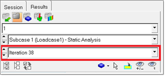
In the Results Browser, select the last
iteration.
From the Results toolbar, click to open the Contour panel.
Under Result type, select Element densities
(s) and
Density.
Set the Averaging method: to
Simple.
Click Apply.
The resulting contours represent the displacement field resulting from
the applied loads and boundary conditions.
In this model, refining the mesh should provide a more discrete solution;
however, for the sake of this tutorial, the current mesh and results
are sufficient.
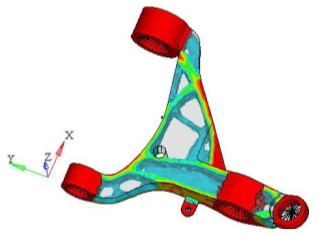
Set Iso Plot of Densities
The iso surface feature can be a very useful tool for post-processing density results from
OptiStruct. For models with solid design
regions, this feature becomes a vital tool for analyzing density
results.
In the Results Browser, verify the last
iteration is still selected.
From the Results toolbar, click to open the Iso Value
panel.
Set the Result type: to Element Densities
(s).
Click Apply.
Change the density threshold.
In the Current value field, enter
0.3.
Under Current value, move the slider.
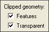
Set Show values to Above.
Under Clipped geometry, select Features
and Transparent.
Figure 2.
Figure 3. Isosurface Plot of Element Densities
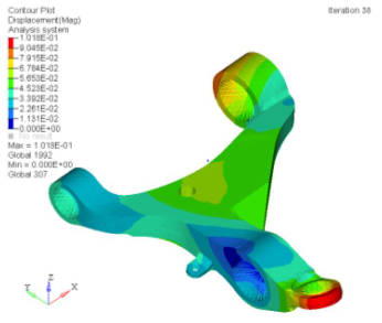
View Contour Plot of Displacements and Stresses
In the top, right of the application, click to proceed to the results of Load Case 1 on page 3.
On the Animation toolbar, set the animation mode to (Linear Static).
On the Results toolbar, click to open the Contour panel.
Set the Result type: to Displacements (v).
Click Apply.
The displacement plot for Iteration 0 displays.
In the Results Browser, set the iteration to the last
iteration.
Figure 4. Displacement Plot for the Last Iteration
A displacement plot for the last iteration displays. The stress results
are also available for the respective iterations. Figure 5. Displacement Contour for the First Loadstep at the Last
Iteration
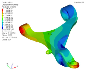
Similarly, view the results for Load Case 2 on page 4.
Figure 6. Displacement Contour for the Second Loadstep at the Last
Iteration
 to open the Contour panel.
 to open the Iso Value
panel.
to open the Iso Value
panel.
 to proceed to the results of Load Case 1 on page 3.
 (Linear Static).