OS-T: 2070 Reduced Model using DMIG
In this tutorial an existing finite element model of a simple cantilever beam is used to demonstrate how to reduce the finite element model using static reduction. You will also perform a topology optimization on the reduced model.
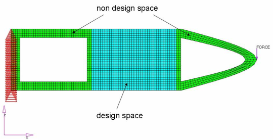
Figure 1. Full Cantilever Beam Model Without Static Reduction
- Objective
- Minimize compliance.
- Constraints
- Upper bound constraint of 40% for the designable volume.
- Design Variables
- The density for each element in the design space.
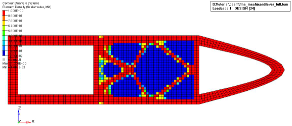
Figure 2. Topology Optimization Results for the Full Cantilever Beam Model
The part to be reduced out of the model through the static reduction model reduction technique is referred to as a superelement. In OptiStruct, ASET or ASET1 Bulk Data Entries are required to indicate the boundary degrees of freedom of a superelement, meaning the set of degrees-of-freedom where the component (being replaced by direct matrix input) connects to the modeled structure. Both the accuracy and the cost of static reduction increase as the number of ASET entries is increased. For example, by using static reduction, the size of the matrix to solve will become smaller, but if the reduced matrix (DMIG) is very dense, then the solution time will become larger than the solution time for the full model where the matrix may be sparse. Hence, the selection of ASET entries is very important in performing an efficient analysis using DMIG.
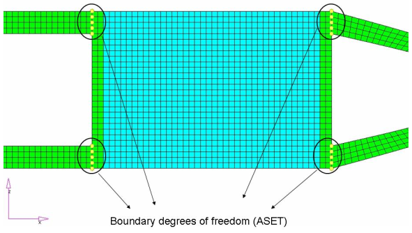
Figure 3. ASET for the Cantilever Beam Model
Launch HyperMesh and Set the OptiStruct User Profile
Open the Model
Generate a Superelement
Create ASETs Load Collector
-
Create a load collector.
-
Create constraints.
-
Using the nodes selector, select boundary nodes.
Figure 4.
-
Using the nodes selector, select boundary nodes.
- Click return to go to the main menu.
Delete Elements Retained in the Subsequent Optimization
-
Draw a window around the elements indicated in Figure 5.
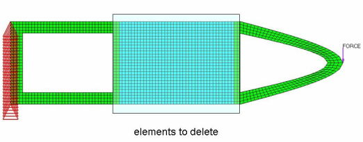
Figure 5.
Define a Parameter to Write out Reduced Matrices to an External File
- On the Analysis page, click the control cards panel.
- In the Card Image dialog, click PARAM.
- Select EXTOUT.
- At the top of the card image, under the EXTOUT, select DMIGPCH.
- Click return to exit PARAM.
- Click return to get back to the main menu.
Save the Database
- From the menu bar, click .
- In the Save As dialog, enter cantilever_dmig.hm for the file name and save it to your working directory.
Submit the Job
-
From the Analysis page, click the OptiStruct
panel.
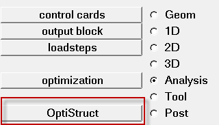
Figure 6. Accessing the OptiStruct Panel
- cantilever_dmig.out
- OptiStruct output file containing specific information on the file setup, the setup of your optimization problem, estimates for the amount of RAM and disk space required for the run, information for each of the optimization iterations, and compute time information. Review this file for warnings and errors.
- cantilever_dmig.stat
- Summary of analysis process, providing CPU information for each step during analysis process.
- cantilever_dmig_AX.pch
- Reduced matrices (DMIG) file.
The matrices are written to the .pch file with the same format as the DMIG Bulk Data Entry. They are defined by a single header entry and one or more column entries. By default, the name of the stiffness matrix is KAAX, the mass is MAAX, and the load is PAX. Since mass matrix is not used in this tutorial, it is not written to .pch file.
The I/O Option Entry, DMIGNAME, provides you with control over the name of the matrices.
Clear the Database
Include the Superelement in the Model
Open the Model
Delete Superelement Part Reduced out using DMIG
-
Draw a window around the elements indicated in Figure 7.
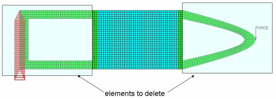
Figure 7.
Set up Topology Optimization with DMIG
- On the Analysis page, click the control cards panel.
-
Define the INCLUDE_BULK control card.
-
Define the K2GG control card.
-
Define the P2G control card.
- Click P2G.
- In the P2G= field, enter PAX.
- Click return to exit the P2G control card.
- Click return to go to the main menu.
Set Up the Optimization
Create Topology Design Variables
- From the Analysis page, click optimization.
- Click topology.
- Select the create subpanel.
- In the desvar= field, enter topo.
- Set type: to PSHELL.
- Using the props selector, select design.
- Click create.
-
Update the design variable's parameters.
- Select the parameters subpanel.
- Toggle minmemb off to mindim=, then enter 1.2.
- Click update.
- Click return.
Create Optimization Responses
- From the Analysis page, click optimization.
- Click Responses.
-
Create the volume fraction response.
- In the responses= field, enter Volfrac.
- Below response type, select volumefrac.
- Set regional selection to total and no regionid.
- Click create.
-
Create the compliance response.
- In the response= field, enter Compl.
- Below response type, select compliance.
- Set regional selection to total and no regionid.
- Click create.
- Click return to go back to the Optimization panel.
Create Design Constraints
- Click the dconstraints panel.
- In the constraint= field, enter VFrac.
- Click response = and select Volfrac.
- Check the box next to upper bound, then enter 0.4.
- Click create.
- Click return to go back to the Optimization panel.
Define the Objective Function
- Click the objective panel.
- Verify that min is selected.
- Click response= and select Compl.
- Using the loadsteps selector, select step.
- Click create.
- Click return twice to exit the Optimization panel.
Save the Database
- From the menu bar, click .
- In the Save As dialog, enter cantilever_opti.hm for the file name and save it to your working directory.
Run the Optimization
- cantilever_opti.hgdata
- HyperGraph file containing data for the objective function, percent constraint violations, and constraint for each iteration.
- cantilever_opti.HM.comp.tcl
- HyperMesh command file used to organize elements into components based on their density result values. This file is only used with OptiStruct topology optimization runs.
- cantilever_opti.HM.ent.tcl
- HyperMesh command file used to organize elements into entity sets based on their density result values. This file is only used with OptiStruct topology optimization runs.
- cantilever_opti.html
- HTML report of the optimization, giving a summary of the problem formulation and the results from the final iteration.
- cantilever_opti.oss
- OSSmooth file with a default density threshold of 0.3. You may edit the parameters in the file to obtain the desired results.
- cantilever_opti.out
- OptiStruct output file containing specific information on the file setup, the setup of the optimization problem, estimates for the amount of RAM and disk space required for the run, information for all optimization iterations, and compute time information. Review this file for warnings and errors that are flagged from processing the cantilever_opti.fem file.
- cantilever_opti.res
- HyperMesh binary results file.
- cantilever_opti.sh
- Shape file for the final iteration. It contains the material density, void size parameters and void orientation angle for each element in the analysis. This file may be used to restart a run.
- cantilever_opti.stat
- Contains information about the CPU time used for the complete run and also the break-up of the CPU time for reading the input deck, assembly, analysis, convergence, and so on.
- cantilever_opti_des.h3d
- HyperView binary results file that contain optimization results.
- cantilever_opti_s#.h3d
- HyperView binary results file that contains from linear static analysis, and so on.
View the Results
Element density results are output to the cantilever_opti_des.h3d file from OptiStruct for all iterations. In addition, Displacement and Stress results are output for each subcase for the first and last iterations by default into cantilever_opti_s#.h3d files, where # specifies the sub case ID.
Review the Contour Plot of the Density Results
- From the OptiStruct panel, click HyperView.
-
From the Results toolbar, click
 to open the Contour panel.
- Set the Result type to Element Densities[s] and Density.
- Set the Averaging method to Simple.
- Click Apply to display the density contour.
-
On the Animation toolbar, click
 to choose the last iteration from the
Simulation list.
to choose the last iteration from the
Simulation list.
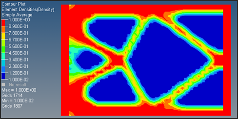
Figure 8.
View an Iso Value Plot of Element Densities
-
From the Results toolbar, click
 to open the Iso Value panel.
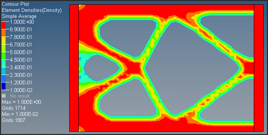
Figure 9.