OS-T: 1530 Bumper Impact

This tutorial demonstrates the setup of a Nonlinear Transient Analysis. In this tutorial, the stopper is defined as rigid.


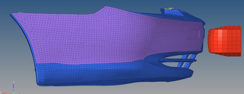
Figure 1. FE Model with Loadcases and Loadstep
The following steps are included:
  • Import the model into HyperMesh
  • Set up nonlinear material.
  • Set up nonlinear analysis
  • View the results in HyperView

Launch HyperMesh and Set the OptiStruct User Profile

  1. Launch HyperMesh.
    The User Profile dialog opens.
  2. Select OptiStruct and click OK.
    This loads the user profile. It includes the appropriate template, macro menu, and import reader, paring down the functionality of HyperMesh to what is relevant for generating models for OptiStruct.

Open the Model

  1. Click File > Open > Model.
  2. Select the Bumper_impact.hm file you saved to your working directory from the optistruct.zip file. Refer to Access the Model Files.
  3. Click Open.
    The Bumper_impact.hm database is loaded into the current HyperMesh session, replacing any existing data. The database only contains geometric and elastic material data.

Set Up the Model

Create TABLES1 Curve

  1. In the Model Browser, right-click and select Create > Curve from the context menu.
    A default load collector displays in the Entity Editor.
  2. For Name, enter TABLES1.
  3. For Card Image, select TABLES1.
  4. In the Model Browser, right-click and select Edit.
  5. In the Table tab of the Curve Editor, enter the numerical data, as shown in Figure 2, where x-axis corresponds to strain and y-axis corresponds to stress.


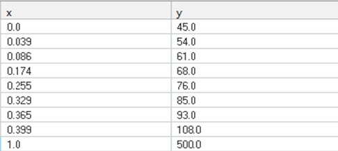
    Figure 2. Define Stress-Strain Curve for the Plastic Material
  6. Close the Curve Editor.

Create the Material

  1. In the Model Browser, right-click and select Create > Material from the context menu.
  2. For Name, enter Plastic_mat.
    A new material, Plastic_mat has beeen created.
  3. Enter the material values next to the corresponding fields.
    1. For E (Young's Modulus), enter 2800.
    2. For NU (Poisson's Ratio), enter 0.2.
    3. For RHO, enter 1.2e-09.
    4. Activate MATX36 and for MATX_type, select MATX36.
      This defines the material properties for piece-wise linear elastic-plastic material.
    5. For EPSMAX, enter 1e+30.
    6. For EPST1, enter 0.4.
    7. For EPST2, enter 0.8.


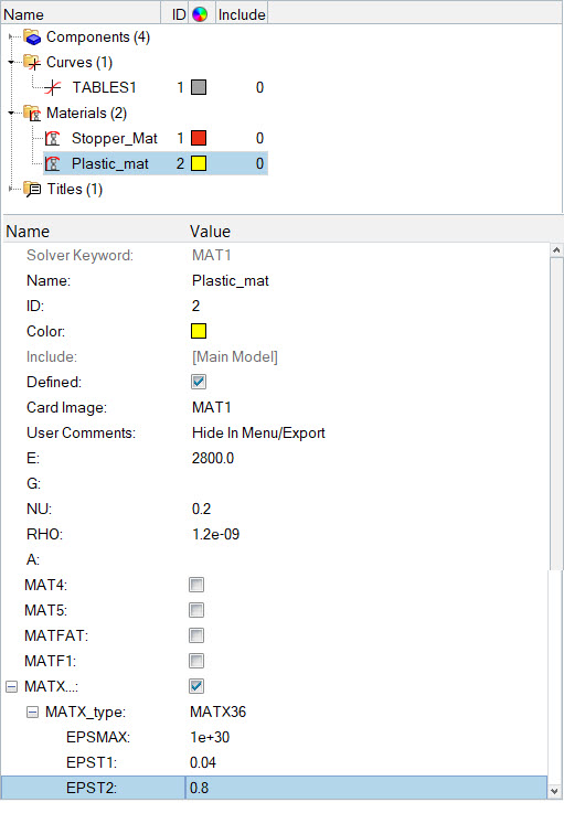
    Figure 3. Define Plastic Material
  4. Click TID and assign TABLES1.

Create the Properties

  1. In the Model Browser, right-click and select Create > Property from the context menu.
    A default PSHELL property displays in the Entity Editor.
  2. For Name, enter Bumper.
  3. For Material, click Unspecified > Material.
  4. In the Select Material dialog, select Plastic_mat and click OK.


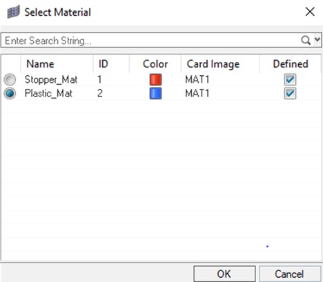
    Figure 4. Select Plastic_mat for the Property Bumper
  5. For T, enter 2.85.
  6. Activate PSHELLX for additional SHELL properties for nonlinear analysis.
  7. For NIP, enter 5.
  8. Activate ITHICK and select VAR to account for thickness changes.
  9. For IPLAS, select NEWT.
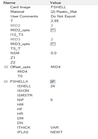

    Figure 5. Property Values for Bumper
    A new property, Bumper has been created as a 2D PSHELLX. Material information is also assigned to this property.
  10. In the Model Browser, Expand the Components folder and click on the component Bumper_T1.
    The component fields display in the Entity Editor.
  11. For Property, click Unspecified > Property.
  12. In the Select Property dialog, select Bumper and click OK.

    The component Bumper_T1 has been updated with a property of the same name and is currently the “Current Component” (see the box in the lower right for Bumper_T1). This component uses the Bumper property definition with a thickness value of 2.85. The material Plastic_mat is referenced by this component.

  13. Assign the Bumper property to the component Bumper_T2 by repeating the steps mentioned previously for Bumper_T1.
  14. In the Model Browser, right-click and select Create > Property from the context menu.
    A default PSHELL property displays in the Entity Editor.
  15. For Name, enter Stopper.


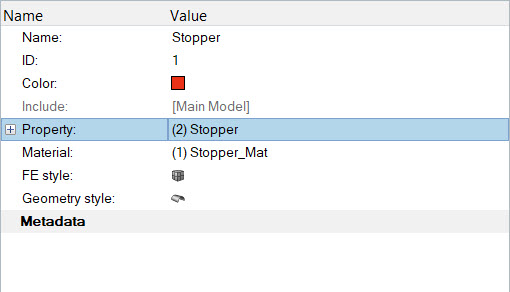
    Figure 6. Property Values for Stopper
  16. For Material, select Stopper_Mat.
  17. For T (thickness of the plate), enter 1.
  18. In the Model Browser, click on the component Stopper.
    The component fields display in the Entity Editor.
  19. For Property, click Unspecified > Property.
  20. In the Select Property dialog, select Stopper and click OK.

Create PCONTX Property

  1. In the Model Browser, right-click and select Create > Property from the context menu.
  2. For Name, enter Contact.
  3. For Card Image, select PCONT.
  4. Activate PCONTX and change PCONTX Type to PCONTX.
  5. For FRIC, enter 0.8.
  6. For IGAP, select VAR.
    This makes the gap varying in both space and time for contact.
  7. For STIF1, enter 4.
    This calculates the stiffness for both Secondary and Main.
  8. For IFORM, select STIFF.
    Defines the type of friction penalty used.

Create Set Segments

The contact surfaces will be defined, which will be used later to define the contact groups.

  1. In the Model Browser, right-click and select Create > Set Segment from the context menu.
  2. For Name, enter Main.
  3. Right-click on the component Stopper and select Isolate Only.
  4. Click Entity IDs to select the elements corresponding to Stopper.
    Note: Make sure to switch the selection panel from faces to elements.
  5. Click elems.
    The selection panel opens.
  6. Click Elements > Displayed.
    This selects all the elements corresponding to the component Stopper.
  7. This creates a Main contact surface with elements corresponding to the Stopper.


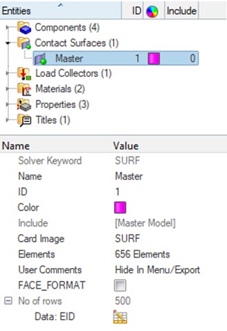
    Figure 7. Create Main Contact Surface
  8. Similarly create a Secondary contact surface with elements corresponding to the components Bumper_T1 and Bumper_T2 by following the steps mentioned above.

Create Contact Groups

Here the contact groups will be defined.

  1. In the Model Browser, right-click and select Create > Group from the context menu.
  2. For Card Image, select CONTACT.
  3. For Name, enter Bumper_contact.
  4. For Property Option, select Property Id.
  5. Expand PID and select Contact surfaces.


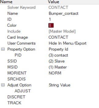
    Figure 8. Create a Contact Group
  6. For Secondary (SSID), select Secondary.
  7. For Main (MSID), select Main.
  8. For MORIENT (Contact Orientation), select NORM.

Apply Loads and Boundary Conditions

In the following steps, SPC constraints are applied on the nodes corresponding to the RBE2. Two SPC’s using SPCADD are added.

Create SPC's Load Collector

  1. In the Model Browser, right-click and select Create > Load Collector from the context menu.
    A default load collector displays in the Entity Editor.
  2. For Name, enter spcl.
  3. Click BCs > Create > Constraints to open the Constraints panel.
  4. Select the nodes 10356, 10357, 10358, 10359, 10360, 10361, 10362, 10363, 10367, 10368 and constrain them in all DOF’s.


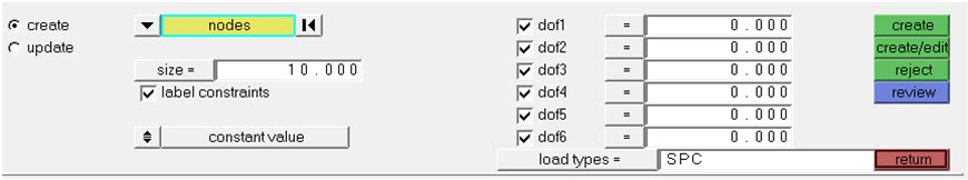
    Figure 9. Constrain All DOFs of Selected Nodes
  5. Click Create.
    This applies the constraints to the selected nodes.
  6. Create another load collector and for Name, enter spc2.
  7. Click Create.
  8. Select the nodes 25744, 25743, 10366 and constrain them in 2, 3, 4, 5, and 6 DOF’s.
  9. In the Model Browser, right-click and select Create > Load Collector from the context menu.
  10. For Name, enter spc_add.
  11. For Card Image, select SPCADD.
  12. Activate SPCADD_Num_Set, enter 2.
    A 2x1 table is created.
  13. Select the spc1 and spc2 created previously.
    spc1 and spc2 are combined into a single card.

Create the Initial Velocity

  1. In the Model Browser, right-click and select Create > Load Collector from the context menu.
    A default load collector displays in the Entity Editor.
  2. For Name, enter Velocity.
  3. Click BCs > Create > Constraints.
  4. For Load Types, select TIC(V).
  5. Select the node 10366.


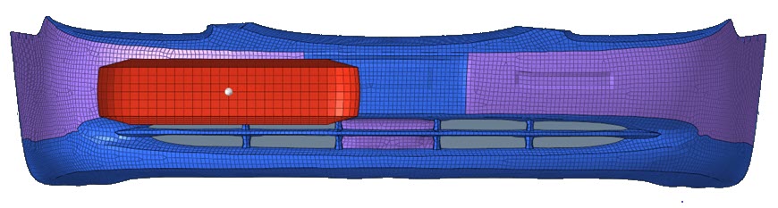
    Figure 10. Apply Initial Velocity
  6. Select dof1 and enter 694.44.


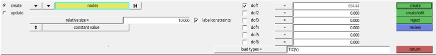
    Figure 11. Define Initial Velocity

Create TSTEP Load Collector

  1. In the Model Browser, right-click and select Create > Load Collector.
  2. For Name, enter TSTEP.
  3. For Card Image, select TSTEP from the drop-down menu.
  4. For N, enter 200.
  5. For DT, enter 0.001.
  6. Click Close.

Create NLPARM Load Collector

  1. In the Model Browser, right-click and select Create > Load Collector.
  2. For Name, enter NLPARM.
  3. Click Color and select a color from the color palette.
  4. For Card Image, select NLPARM from the drop-down menu.
  5. For NINC, enter 500.
  6. For DT, enter 0.001.
  7. For MAXITER, enter 80.
  8. For CONV, select PW.
  9. For TTERM, enter 0.1.
  10. For EPSP, enter 0.001.
  11. For EPSW, enter 1e-6.

Create NLOUT Load Collector

  1. In the Model Browser, right-click and select Create > Load Collector.
  2. For Name, enter NLOUT.
  3. For Card Image, select NLOUT from the drop-down menu.
  4. For NINT, enter 100.

Define Output Control Parameters

  1. From the Analysis page, select control cards.
  2. Click on GLOBAL_OUTPUT_REQUEST.
  3. Below DISPLACEMENT, ELFORCE, STRESS and STRAIN, set Option to Yes.
  4. Click return twice to go to the main menu.

Create DTI, UNITS

  1. From the menu bar, click Setup > Create > Control Cards to open the Control Cards panel.
  2. Click DTI_UNITS.
  3. Define the unit system, as shown in Figure 12.


    Figure 12.
  4. Click return twice to return to the main menu.

Create Load Steps

  1. In the Model Browser, right-click and select Create > Load Step.
    A default load collector displays in the Entity Editor.
  2. For Name, enter Bumper_impact.
  3. For Type, select Nonlinear transient from the drop-down menu.
  4. For SPC, select spcadd.
  5. For TSTEP, select tstep.
  6. For NLPARM(LGDISP), select nlparm.
  7. For DLOAD, select dload from the list of load collectors.
  8. For NLADAPT, select NLAdapt from the list of load collectors.
  9. For NLOUT, select NLout.
  10. Under SUBCASE OPTION, toggle ANALYSIS, and select TYPE DTRAN.
  11. Activate NLMON and select nlmon.
  12. In the SPC Select Loadcol dialog, select spc_add from the list of load collectors and click OK.
    This selects the boundary conditions created above.
  13. In the IC Select Loadcol dialog, select Velocity from the list of load collectors and click OK.
    This selects the boundary conditions created above.
  14. Similarly select the TSTEP, NLPARM_LGDISP, and NLOUT and assign respective load collectors.

Submit the Job

  1. From the Analysis page, click the OptiStruct panel.

    OS_1000_13_17
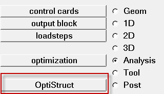
    Figure 13. Accessing the OptiStruct Panel
  2. Click save as.
  3. In the Save As dialog, specify location to write the OptiStruct model file and enter bumper_impact.hm for filename.
  4. Click Save.
    The input file field displays the filename and location specified in the Save As dialog.
  5. Set the export options toggle to all.
  6. Set the run options toggle to analysis.
  7. Click OptiStruct to submit the job.

View the Results

  1. Once you receive the message Process completed successfully in the command window, click HyperView.
  2. Open the results and plot the displacement and the von Mises stress contour at 100% load.
  3. On the toolbar, click resultsContour-16 (Contour).
  4. Under Result type, from the first drop-down menu, select Element Stresses (2D & 3D)(t).
  5. Under Result type, from the second drop-down menu, select vonMises.


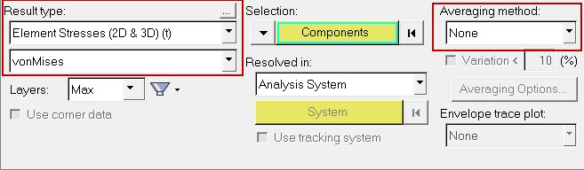
    Figure 14. Contour Panel
  6. Verify that the fields in the Contour panel match those in Figure 14 and click Apply.


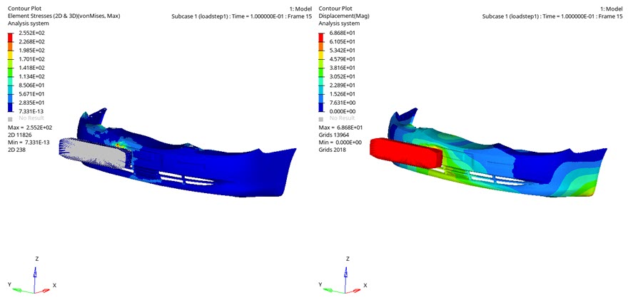
    Figure 15. Displacement and Stress Result for the Analysis