OS-T: 1580 NLSTAT Analysis of Arthritic Finger
This tutorial demonstrates how to carry out nonlinear implicit analysis in OptiStruct involving hyperelastic material and contact.
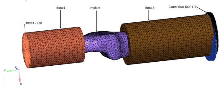
Figure 1. FE Model
- One with Tie contacts
- One with Node2Surface contacts
Launch HyperMesh and Set the OptiStruct User Profile
Open the Model
Set Up the Model
Create Curves
Here you will create the curves for the hyperelastic material.
-
Click on the Table icon
 next to the
Data field and enter the X (strain) and Y (stress) values:
next to the
Data field and enter the X (strain) and Y (stress) values:
Table 1. Simple Tension Compression Data Values X (Strain) Y (Stress) 1.1338 1.5506 1.2675 2.4367 1.3567 3.1013 1.6242 4.2089 1.8917 5.3165 2.1592 5.981 2.4268 6.8671 3.051 8.8608 3.586 10.6329 4.0318 12.4051 4.7898 16.1709 5.3694 19.9367 5.8153 23.481 6.172 27.4684 6.4395 31.0127 6.707 34.557 6.9299 38.3228 7.0637 42.0886 7.1975 45.6329 7.3312 49.3987 7.465 53.1646 7.5541 56.9304 7.6433 64.2405
Create the Materials
This step requires creating the hyperelastic behavior of the implant material and the bone material.
- In the Model Browser, right-click and select from the context menu.
- For Name, enter MATHE_2.
- Click Color and select a color from the color palette.
- For Card Image, select MATHE from the drop-down menu.
- For MODEL, select ABOYCE from the drop-down menu.
- For TAB1, select load-curve (TABLES1100) created in Table 1.
- For TAB2, select load-curve (TABLES1200) created in Table 2.
- For TAB4, select load-curve (TABLES1400) created in Table 3.
- For TABD, select load-curve (TABLES1500) created in Table 4.
- In the Model Browser, right-click and select .
- For Name, enter Bone.
- Click Color and select a color from the color palette.
- For Card Image, select MAT1 from the drop-down menu.
- For E, enter 14800.
- For NU, enter 0.3.
Create IMPLANT Property
The Implant property is created here.
- In the Model Browser, right-click and select from the context menu.
- For Name, enter Implant.
- Click Color and select a color from the color palette.
- For Card Image, select PLSOLID from the drop-down menu, and click Yes to confirm.
- For Material, select .
- In the Select Material dialog, select MATHE_2 from the list of materials and click OK.
Create BONE Property
Now you will create the Bone property.
- In the Model Browser, right-click and select from the context menu.
- For Name, enter Bone.
- Click Color and select a color from the color palette.
- For Card Image, select PSOLID from the drop-down menu and click Yes.
- For Material, click .
- In the Select Material dialog, select Bone from the list of materials and click OK.
Create PCONT Property
- In the Model Browser, right-click and select from the context menu.
- For Name, enter Pcont.
- Click Color and select a color from the color palette.
- For Card Image, select PCONT from the drop-down menu and click Yes.
- For STIFF_REAL_VAL, select STIFF = HARD.
- For MU1, enter 0.3.
Assign Properties
In this step, you will assign the properties to the respective components.
-
In the Model Browser, click and enter the data, as shown below:
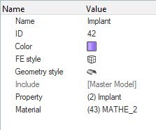
Figure 2. -
Click and enter the data, as shown below:
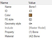
Figure 3. -
Click and enter the data, as shown below:
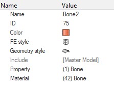
Figure 4.
Apply Loads and Boundary Conditions
Create IMPLANT Set Segment
Here you will select the Implant faces and define the contact surface.
-
In the second drop-down list, select faces.
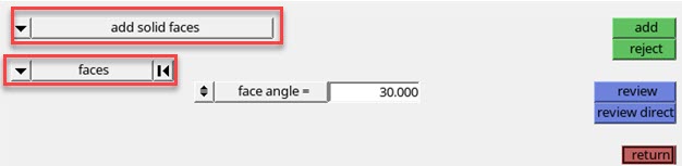
Figure 5. Selection Panel
Create BONE Set Segment
Here you will select the Bone1 and Bone2 faces and define the contact surface.
-
In the second drop-down list, select faces.
Figure 6. -
Select the inside faces of Bone1 and Bone2 (selected faces are blue), as shown
below:
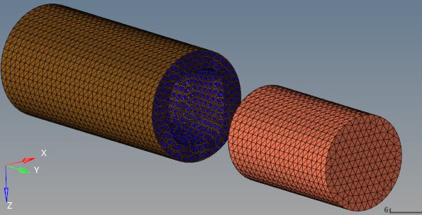
Figure 7. Bone1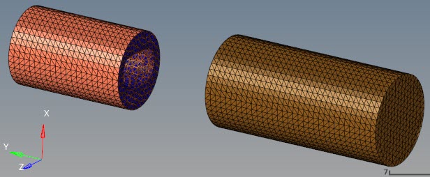
Figure 8. Bone2
Create Contacts
Here you will create a TIE contact and a N2S contact.
- In the Model Browser, right-click and select .
- For Name, enter Contact.
- Click Color and select a color from the color palette.
- For Card Image, select TIE from the drop-down menu and click Yes.
- For SSID, select and select Implant1.
- For MSID, select and select Bone1.
- In the Model Browser, right-click and select .
- For Name, enter Contact.
- Click Color and select a color from the color palette.
- For Card Image, select CONTACT from the drop-down menu and click Yes.
- Toggle Property Option, and for PID, select Pcont.
- For SSID, select and select Implant1.
- For MSID, select and select Bone1.
Create NLPARM Load Collector
The nonlinear implicit parameters are defined.
- In the Model Browser, right-click and select .
- For Name, enter nlParm.
- Click Color and select a color from the color palette.
- For Card Image, select NLPARM from the drop-down menu.
Create NLADAPT Load Collector
- In the Model Browser, right-click and select .
- For Name, enter NLAdapt.
- Click Color and select a color from the color palette.
- For Card Image, select NLADAPT from the drop-down menu.
- For NCUTS, enter 25.
Create NLMON Load Collector
- In the Model Browser, right-click and select .
- For Name, enter NLMon.
- Click Color and select a color from the color palette.
- For Card Image, select NLMON from the drop-down menu.
- For ITEM, select DISP.
- For INT, select ITER.
Create NLOUT Load Collector
- In the Model Browser, right-click and select .
- For Name, enter NLOUT.
- Click Color and select a color from the color palette.
- For Card Image, select NLOUT from the drop-down menu.
- For NINT, enter 10.
- Activate SVNONCNV and select YES for the VALUE.
Create CNTSTB Load Collector
- In the Model Browser, right-click and select .
- For Name, enter cntstb.
- Click Color and select a color from the color palette.
- For Card Image, select CNTSTB from the drop-down menu.
- For S0, enter 0.01.
- For S1, enter 1e-05.
Create BCS Load Collector
Here the boundary condition is defined.
-
Select all the nodes of the Bone1 rear side face and activate all DOF and enter
0 for each.
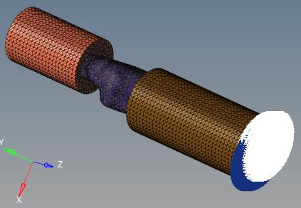
Figure 9.
Create Force
-
For elem types, enter RBE2 and click
create.
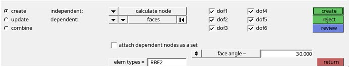
Figure 10. -
For load types, enter FORCE.
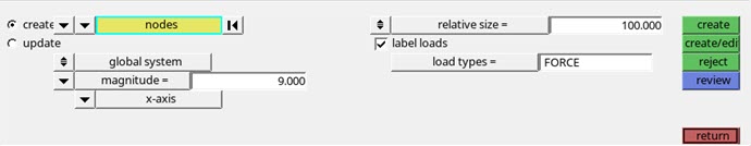
Figure 11.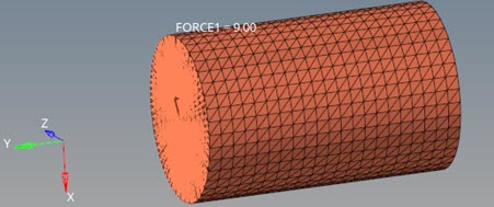
Figure 12.
Create Load Step
The nonlinear static load step is created.
- In the Model Browser, right-click and select .
- For Name, enter load.
- Click Color and select a color from the color palette.
- For Analysis type, select Nonlinear static from the drop-down menu.
- For SPC, select Bcs from the list of load collectors.
- For LOAD, select Force.
- For NLPARM, select NLPARM.
- For NLADAPT, select NLAdapt.
- For NLOUT, select NLout.
- For CNTSTB, select cntstb.
Define Output Control Parameters
- From the Analysis page, select control cards.
- Click on GLOBAL_OUTPUT_REQUEST.
- Select ELFORCE, SPCF, STRAIN, and STRESS.
- In the control cards page, click GAPPRM, PARAM and FORMAT.
- Click return twice to go to the main menu.
Submit the Job
-
From the Analysis page, click the OptiStruct
panel.
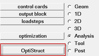
Figure 13. Accessing the OptiStruct Panel
View the Results
-
On the toolbar, click
 (Contour).
-
Under Result type, from the second drop-down menu, select
vonMises.
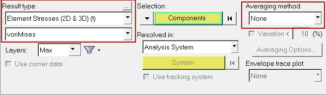
Figure 14. Contour Panel -
Verify that the fields in the Contour panel match those in
Figure 14 and click
Apply.
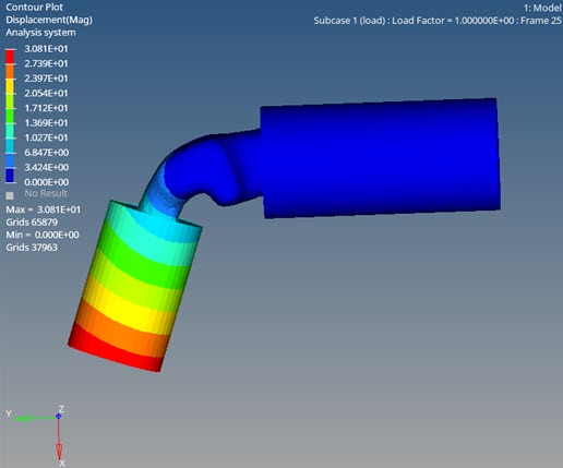
Figure 15. Contour of Displacement in Bone and Implant subject to Loading. TIE Contact Results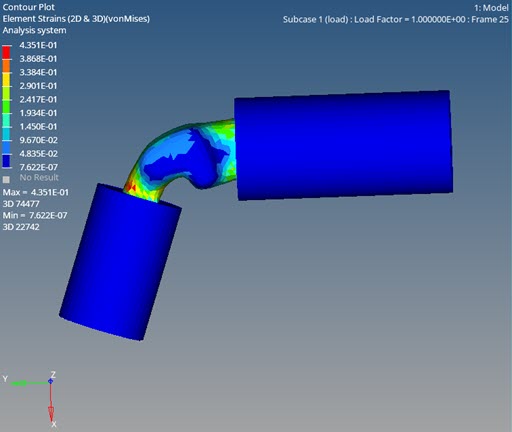
Figure 16. Contour of Element Strains in Bone and Implant subject to Loading. TIE Contact Results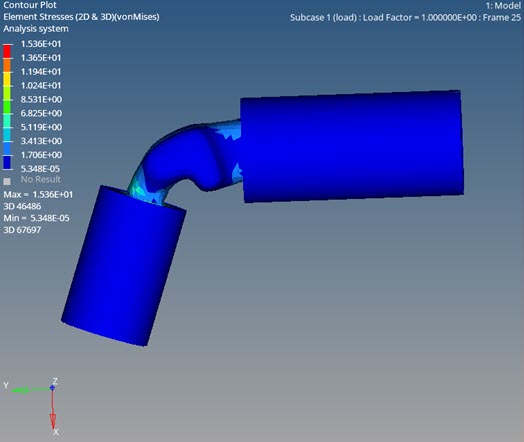
Figure 17. Contour of Element Stresses in Bone and Implant subject to Loading . TIE Contact Results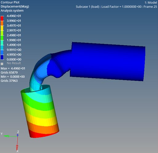
Figure 18. Contour of Displacement in Bone and Implant subject to Loading. N2S Contact Results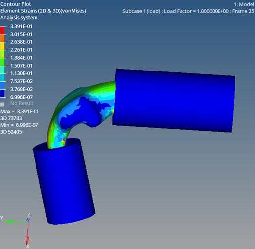
Figure 19. Contour of Element Strains in Bone and Implant subject to Loading. N2S Contact Results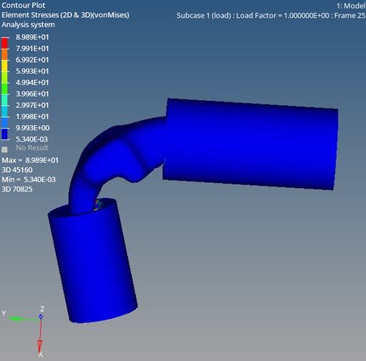
Figure 20. Contour of Element Stresses in Bone and Implant subject to Loading . N2S Contact Results