Soft Soil Tire Model
The Altair Soft Soil Tire model provides a way to simulate the dynamic behavior of a tire on a surface that is compressible such as clay, dry sand, regolith, and ice-covered snow.
Sample tire and soil property files are located in the installation here: <Installation>\hwdesktop\hw\mdl\autoentities\properties\Tires\ALTAIR_SOFTSOIL
Theoretical Approach
In the current tire model, the deformations of the soil which eventually lead to the corresponding (normal and shear) stresses are considered as two independent effects. Specifically, the strength of the soil is considered in the vertical direction (pressure-sinkage relationship) as well as in the horizontal direction (shear stress-shear displacement relationship).
Pressure-Sinkage Relationship
If a terrain is assumed to be homogeneous, its pressure-sinkage relationship (the result of the plate-sinkage test) may take one of the forms which are shown in Figure 1, and it may be characterized by the following empirical equation proposed by Bekker. [1]

Where  is pressure,
  is the width of the rectangular contact patch area,
  is sinkage, and
  , and
, and  , are pressure-sinkage related parameters.

Soil Failure
There is a variety of criteria proposed for the failure of soils. One of the most widely
used is the Mohr-Coulomb criterion which states that the maximum shear strength  of the soil is:
Where  is the apparent cohesion,
  is the normal stress, and
  is the angle of internal shearing resistance of the material. The
aforementioned parameters can be derived with a shear test for different pressures, as shown
in Figure 2:
is the angle of internal shearing resistance of the material. The
aforementioned parameters can be derived with a shear test for different pressures, as shown
in Figure 2:

Tire-Road Interaction
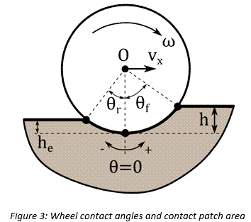
Contact Patch Area
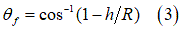
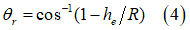
In the case of a moving wheel, the contact patch area can be determined as a function of
sinkage  , the tire’s radius
  , and elastic sinkage
  using the following equations:
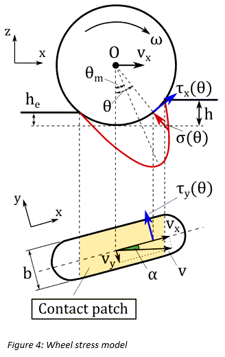
Normal Stress
Using the pressure-sinkage relationship proposed by Bekker (Eq. (1)), the tire normal
stress distribution can be calculated as a function of wheel angle  [2]. Specifically,

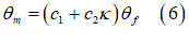
where b is the tire’s width. Moreover,  is the wheel angle at which the normal stress is maximized [2]
and can be determined as:
is the wheel angle at which the normal stress is maximized [2]
and can be determined as:
In the above equation,  and
and  are parameters that depend on the wheel-soil interaction,
  is the longitudinal slip, and
  is tire entry angle.
Furthermore, Eq. (5) can be modified in order to account for the contribution of soil damping [3]. In that case, the normal stress distribution is given by:
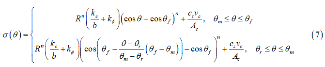
Where  is the soil damping,
  is soil’s compression rate/velocity, and
  is the contact patch area.
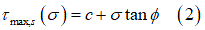
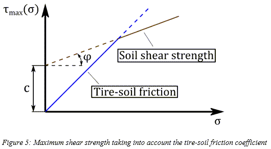
Influence of the Coefficient of Friction
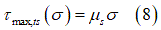
As already mentioned, the maximum shear strength of the soil  can be calculated using Eq. (2) based on the Mohr-Coulomb failure
criterion. In addition, the maximum shear strength between the tire and the soil
can be calculated using Eq. (2) based on the Mohr-Coulomb failure
criterion. In addition, the maximum shear strength between the tire and the soil  can be approximated as a function of the pressure
  and the friction coefficient
 :
:
Consequently, the minimum shear strength (soil–tire and internal soil) is used for the shear stress calculation in order to account for the friction between the tire and the soil [4].

The friction coefficient normally has a value between 0.3 and 1.0 and largely depends on
the material of the tire and the water content of the soil [4].
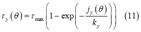
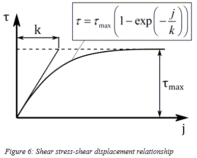
Shear Stress
The shear stresses  and
and  are calculated using identical expressions [5], [6].

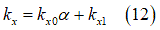
In the above equations,  and
and  represent the shear deformation modules, which are provided by
the following equations:
represent the shear deformation modules, which are provided by
the following equations:
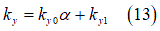
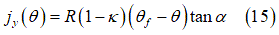
Where  is the slip angle of the tire. Moreover, the soil deformations
 and
and  can be formulated as functions of the wheel angle
  [2], [7]:

 and can be found in the following publications:
- ‘Terramechanics-based Model for Steering Maneuver of Planetary
Exploration Rovers on Loose Soil’ by G. Ishigami and K. Yoshida,
2007 [5]
 [m]
[m]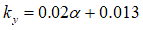 [m]
[m]
- ‘Soil-tire interaction analysis for agricultural tractors: Modeling of
traction performance and soil damage’ by A. Battiato, 2014 [8]
 [m] for clay
 [m] for clay loam
 [m] for silty loam
 [m] for loamy sand
- ‘Terramechanics-based analysis for slope climbing capability of a
lunar/planetary rover’ by K. Yoshida and G. Ishigami, 2004 [9]
 [m] for dry sand
 [m] for regolith simulant
- ‘Analysis of off-road tire-soil interaction through analytical and
finite element methods’ by H. Li, 2013 [3]
 [m]
[m] [m]
[m]
Moreover, according to Wong [10], based on experimental data collected, the value of
ranges from 0.01 [m] for firm sandy terrain to 0.025
[m] for loose sand and is approximately 0.006 [m] for clay at maximum compaction.
For undisturbed fresh snow, the value of varies in the range from 0.025 [m] to 0.05 [m].
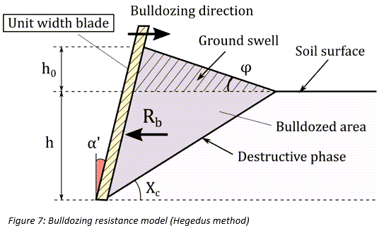
Bulldozing Resistance
Bulldozing resistance is developed when a soil mass is displaced by the wheel. Regarding
lateral forces, due to tire’s sinkage, a bulldozing force which acts on the side of the
wheel must be added to the shear force exerted on the contact patch due to the tangential
stresses  . In this tire model, the Hegedus resistance estimation method
[11] is used in order to calculate the bulldozing force. As depicted in Figure 7, a
bulldozing resistance
. In this tire model, the Hegedus resistance estimation method
[11] is used in order to calculate the bulldozing force. As depicted in Figure 7, a
bulldozing resistance  is developed per unit width of a blade, as the blade moves toward
the soil, given by the equation:
is developed per unit width of a blade, as the blade moves toward
the soil, given by the equation:
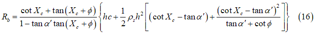
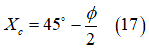
Where  is the soil density. Moreover, the destructive angle
  , based on Bekker’s theory [12], can be approximated as:
Tire Deformability
In order to account for tire deformability, a larger substitute circle is used to describe the contact patch between the tire and the soil [1], [4], [13], as depicted in Fig. 8. In order to calculate the diameter of the substitute circle, an iterative procedure is followed until the soil vertical reaction force and the tire vertical force are balanced. The former is calculated from an integration of the normal and shear stresses in the contact patch area, while for the latter the vertical tire stiffness is used along with the tire’s deflection. More specifically,

The last three equations are solved iteratively until:
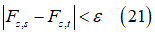
Where the tolerance  is a function of the tire’s maximum vertical load. If the tire’s deformation is
negligible, you can set the boolean flag RIGID_MODE= 'TRUE' in the tire’s
parameter file in order to simplify and accelerate the calculation of the vertical force
is a function of the tire’s maximum vertical load. If the tire’s deformation is
negligible, you can set the boolean flag RIGID_MODE= 'TRUE' in the tire’s
parameter file in order to simplify and accelerate the calculation of the vertical force
 . Specifically, no iterations are required since only Eq. (18) is
used in which the quantities
. Specifically, no iterations are required since only Eq. (18) is
used in which the quantities  and
and  are replaced by
  and
and  respectively. By default, the aforementioned boolean flag is set
to FALSE, making use of the substitute circle concept and thus providing
an increase accuracy.
respectively. By default, the aforementioned boolean flag is set
to FALSE, making use of the substitute circle concept and thus providing
an increase accuracy.

Multipass Effect
For the multipass effect, the response of the soil to repetitive normal load needs to be
established. Specifically, the mathematical description of the normal pressure distribution
must be modified in cases of existing pre-compaction of the soil. As shown in Fig. 9, the
normal pressure distribution will be comprised initially from an elastic part  , which is equal to the elastic (unloading) sinkage that a
previous tire has created. Then the pressure-sinkage relationship continues according to Eq.
(1). Finally, an unloading elastic part
, which is equal to the elastic (unloading) sinkage that a
previous tire has created. Then the pressure-sinkage relationship continues according to Eq.
(1). Finally, an unloading elastic part  is encountered.
As already mentioned, one part of the induced soil deformation is elastic (elastic sinkage), and the remaining part (plastic sinkage) is irreversible. The elastic part is provided by the equation:
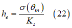
Where  is the soil elastic stiffness.
If the multipass effect is not of interest, you can set the boolean flag MULTIPASS='FALSE' in the road data file. By default, this flag is set to TRUE in order to enable updating the road data.

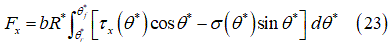
Tire Forces
Longitudinal force:
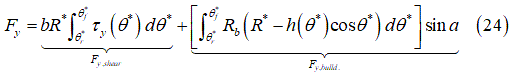
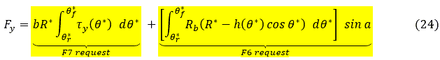
Lateral force:
Overturning moment:
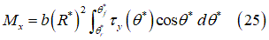
Rolling resistance moment:
Self-aligning moment:
The above equations are used when tire’s deformability is taken into account. When the
RIGID_MODE flag is set to TRUE, the quantities  and
and  are replaced by and respectively.
It should be mentioned that the above integrals are calculated numerically. You can change the number of points used for the calculation of these integrals by setting the integer variable NODES=x in the PARAMETERS block of the road data file in order to obtain an improved accuracy. An estimation of approximately 3-5 integration points should be enough in most cases.
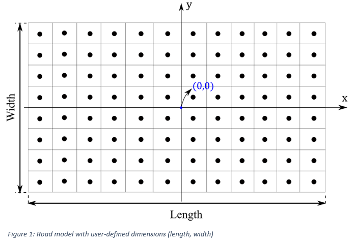
Road Modeling
In this tire model, the road surface is represented as a regular grid of deformable springs
in the vertical (z-axis) direction, as depicted in Fig. 10. Using this approach, each spring
represents a small road patch for which the necessary information can be stored. Typical
values include the soil parameters, the soil elevation (z coordinate) as well as information
regarding the compaction of the soil  , as a function of
  and
and  coordinate. Moreover, the information stored for each region is
set independently of the other springs. In addition, the grid spacing is set automatically
based on the minimum tire width of the model.
coordinate. Moreover, the information stored for each region is
set independently of the other springs. In addition, the grid spacing is set automatically
based on the minimum tire width of the model.

Contact Method
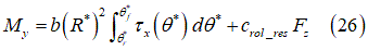
There are two available contact methods in the soft-soil tire model. The required outputs
for both contact models are the soil elevation and the local inclinations of the road
surface  . The default option is to collect all the spring regions that
belong to the contact patch area and use an averaging process to calculate a representative
value for the soil elevation. This is accomplished through a Radial Basis Function (RBF)
interpolation. Moreover, using this approach, the local inclinations of the road surface
can be calculated in an efficient way [14].
. The default option is to collect all the spring regions that
belong to the contact patch area and use an averaging process to calculate a representative
value for the soil elevation. This is accomplished through a Radial Basis Function (RBF)
interpolation. Moreover, using this approach, the local inclinations of the road surface
can be calculated in an efficient way [14].
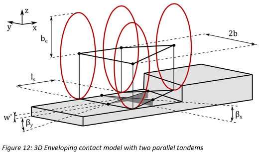
The second option is to use the 3D Enveloping contact method [15], [16]. This contact model
can provide improved accuracy in cases of short wavelengths (sharp steps) in road height.
However, it is a more computationally expensive approach in comparison to the aforementioned
RBF interpolation method. The core idea is to use a series of ellipses to scan the road
profile and produce an effective road plane which is defined by three quantities. Namely,
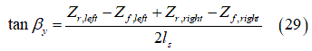
the modified effective height  , the effective forward slope
  and the effective road camber angle
  . The simplest form of this contact model is depicted in Fig. 12,
for which:
. The simplest form of this contact model is depicted in Fig. 12,
for which:
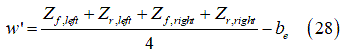

Where  is the cam center height.
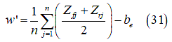
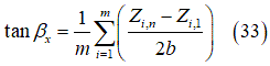
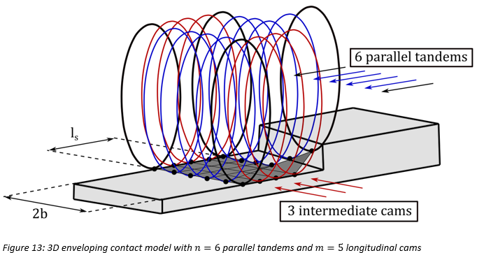
In general, two parallel tandems are not sufficient to obtain accurate results for sharp irregularities. Therefore, more parallel tandems as well as intermediate cams are added, as depicted in Fig. 13. Intermediate cams between the left and right sides are not necessary since their contribution cancel out when calculating the effective road camber angle [15]. The same equations as presented for the previous simple enveloping contact model apply again, but now extended for the case of multiple parallel tandems and intermediate cams. Specifically,

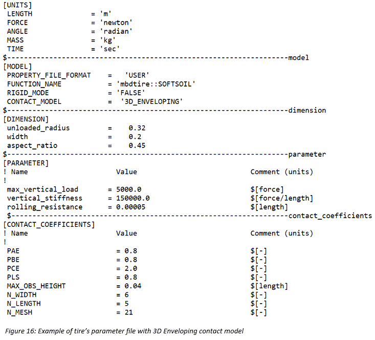
| Parameter | Description | Units |
|---|---|---|
| PAE | Half ellipse’s length/unloaded radius | - |
| PBE | Half ellipse’s height/unloaded radius | - |
| PCE | Ellipse’s exponent | - |
| PLS | Tandem base length factor | - |
| MAX_OBS_HEIGHT | Maximum obstacle height | Length |
| N_WIDTH | Number of cams along the contact width | - |
| N_LENGTH | Number of cams along the contact length | - |
| N_MESH | Number of ellipse’s discretization points | - |
It should be emphasized that you can set which of the tires (if any) will use the 3D Enveloping contact method. This means that in a model both tires that use the Radial Basis Function (RBF) interpolation method as well as tires that use the 3D Enveloping contact model can co-exist leading in an optimal combination of accuracy and computational efficiency. This can be accomplished through different tire parameters files depending on the application’s needs.
Transient Model
A transient model, as described in [16], has been incorporated in this tire model in order
to enhance its behavior at low velocities. The core idea is that the contact point is
connected to the wheel rim with a longitudinal and a lateral spring, which represent the
compliance of the tire’s carcass. Specifically, as depicted in Fig. 14, the contact point
![]() is connected using these springs to the wheel slip point
is connected using these springs to the wheel slip point ![]() , which is attached to the wheel rim. The difference of the slip
velocities of the points
, which is attached to the wheel rim. The difference of the slip
velocities of the points ![]() and
and ![]() produce the carcass springs’ deflection. Subsequently, for the
time derivatives of the longitudinal and lateral deflection,
produce the carcass springs’ deflection. Subsequently, for the
time derivatives of the longitudinal and lateral deflection, ![]() and
and ![]() respectively, it holds that:
respectively, it holds that:
![]()
![]()
After proper transformation [16], the previous set of Ordinary Differential Equations (ODE’s) take the following form:
![]()
![]()
Where ![]() and
and ![]() are the contact patch slip quantities which will be used instead
of
are the contact patch slip quantities which will be used instead
of ![]() and
and ![]() respectively and
respectively and ![]() are the longitudinal and lateral relaxation length.
are the longitudinal and lateral relaxation length.
Due to the fact that at zero forward velocity an undamped vibration might occur using the previous equations, an artificial damping has been added in the transient model [16]. In that case, the damped contact patch slip quantity:
![]()
is used instead of ![]() . Finally, the transient model has been extended in order to cover
the non-linear range of the slip characteristics. Specifically, the restricted fully
non-linear model [16] has been implemented. For this model, Eq. (36) still applies, but the
relaxation length is replaced by the quantity:
. Finally, the transient model has been extended in order to cover
the non-linear range of the slip characteristics. Specifically, the restricted fully
non-linear model [16] has been implemented. For this model, Eq. (36) still applies, but the
relaxation length is replaced by the quantity:
![]()
Where ![]() is the value of the relaxation length at
is the value of the relaxation length at ![]() ,
, ![]() represents the minimum value of the relaxation length, which is
introduced to avoid numerical difficulties and
represents the minimum value of the relaxation length, which is
introduced to avoid numerical difficulties and ![]() is the slip value where the peak force is encountered. It should
be noted that, similar equations to Eq. (38) and Eq. (39) apply also for the calculation of
the lateral contact patch slip quantity
is the slip value where the peak force is encountered. It should
be noted that, similar equations to Eq. (38) and Eq. (39) apply also for the calculation of
the lateral contact patch slip quantity ![]() .
.
It is possible that, during low velocity maneuvers, the solver will encounter convergence difficulties. If this is the case, you should try to change the default simulation parameters. Specifically, decreasing the maximum time step and/or the maximum order might help fix the issue.
Statics
In this tire model, the vertical force  depends on the value of the longitudinal slip
  .
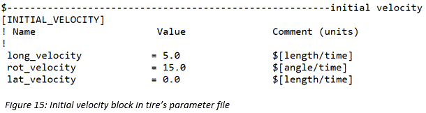
As a consequence, in case of significant initial longitudinal slip the user should define
the tire’s initial longitudinal, lateral, and rotational velocity in an
INITIAL_VELOCITY block of the tire’s parameter file for an accurate
calculation of the static equilibrium position. If this is not the case, the default (zero)
values are used for these velocities.
.
As a consequence, in case of significant initial longitudinal slip the user should define
the tire’s initial longitudinal, lateral, and rotational velocity in an
INITIAL_VELOCITY block of the tire’s parameter file for an accurate
calculation of the static equilibrium position. If this is not the case, the default (zero)
values are used for these velocities.
Soil Library
A soil library with ready-to-use road data files for a variety of soils has been created based on a various information collected from relevant books and papers. This soil library can be found in the installation of the software.
Tire Parameters
- Unloaded radius
- Width
- Vertical stiffness
- Tire (internal) rolling resistance coefficient
- Maximum vertical load
- Rigid mode (Optional. Default=FALSE)
- Contact method (Optional. Default=Radial Basis Function interpolation)
- Initial velocities (Optional)
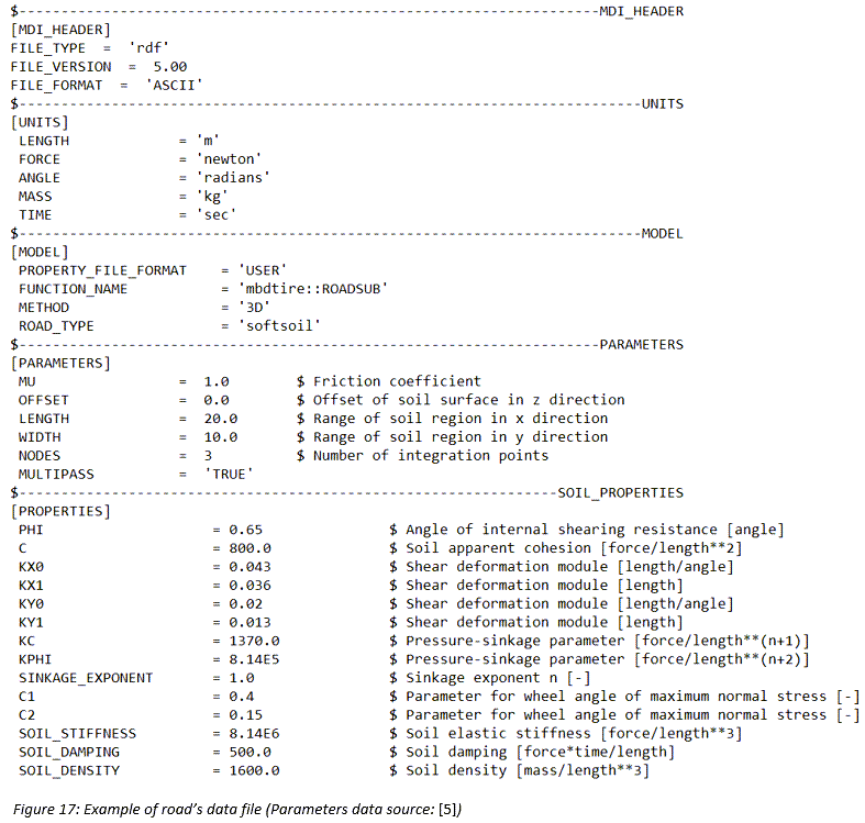
Property File Examples
Tire Parameters File
Road Data File
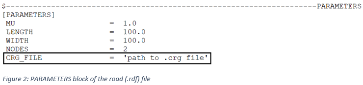
CRG Road Data File
By default, a flat road model with the user-defined dimensions (length, width) is created using the soft-soil tire model (see Fig. 1). In order to represent complex terrain geometries, this tire model enables the use of .crg files. For this, the attribute CRG_FILE=’path to .crg file’ needs to be set in the PARAMETERS block of the road (.rdf) file (see Fig. 2). It should be mentioned that the obstacles are still superimposed on the existing road geometry. Finally, if the specified .crg file cannot be found, the simulation proceeds using a flat road model.
MotionSolve Output Requests
- F2 – Plastic sinkage
- Permanent compression of soil due to tire dynamics (Length h-he in Figure 3).
- F3 – Long Resistance
- Force contribution of the soil normal stress to the longitudinal force (refer to equation 23).
- F4 – Long Shear
- Force contribution of the soil shear stress to the longitudinal force (refer to
equation 23).

- F6 – Lat bulldozing
- The Bulldozing force acting on the tire’s lateral side (refer to equation 24)
- Lat Shear force
- Force contribution of the soil shear stress to the lateral force (refer to equation
24).
- F8 – Tire Sinkage
- Soil compression at tire contact patch (length h in figure 3).
References
[1] M.G.Bekker, Introduction to terrain-vehicle systems. part i: The terrain. part ii: The vehicle. Michigan Univ Ann Arbor, 1969.
[2] J.Y.Wong and A.R.Reece, “Prediction of rigid wheel performance based on the analysis of soil-wheel stresses Part I. Performance of driven rigid wheels,” J. Terramechanics, vol. 4, no. 1, pp. 81–98, 1967.
[3] Hao-Li, “Analysis of Off-Road Tire-Soil Interaction through Analytical and Finite Element Methods,” Technischen Universität Kaiserslautern, 2013.
[4] C. Harnisch, B. Lach, R. Jakobs, M. Troulis, and O. Nehls, “A new tyre-soil interaction model for vehicle simulation on deformable ground,” Veh. Syst. Dyn., vol. 43, no. SUPPL., pp. 384–394, 2005, doi: 10.1080/00423110500139981.
[5] I. Genya, M. Akiko, N. Keiji, and Y. Kazuya, “Terramechanics-Based Model for Steering Maneuver of Planetary Exploration Rovers on Loose Soil,” J. F. Robot., vol. 7, no. PART 1, pp. 81–86, 2015, doi: 10.1002/rob.
[6] Z.Janosi, “The analytical determination of drawbar pull as a function of slip for tracked vehicles in deformable soils,” in Proc. of 1st Int. Conf. of ISTVS, 1961.
[7] K. Yoshida and G. Ishigami, “Steering characteristics of a rigid wheel for exploration on loose soil,” 2004 IEEE/RSJ Int. Conf. Intell. Robot. Syst., vol. 4, no. January 2004, pp. 3995–4000, 2004, doi: 10.1109/iros.2004.1390039.
[8] A.Battiato, “Soil-tyre interaction analysis for agricultural tractors: modelling of traction performance and soil damage,” 2014.
[9] K. Yoshida, N. Mizuno, G. Ishigami, and A. Miwa, “Terramechanics-based analysis for slope climbing capability of a lunar/planetary rover,” in 24th Int. Symp. on Space Technology and Science, 2004.
[10] J.Y.Wong, Theory of ground vehicles. John Wiley & Sons, 2008.
[11] E.Hegedus, “A simplified method for the determination of bulldozing resistance,” 1960.
[12] M.G.Bekker, Off-the-road locomotion. The University of Michigan Press, 1960.
[13] I. C. Schmid, “Interaction of vehicle and terrain results from 10 years research at IKK,” J. Terramechanics, vol. 32, no. 1, pp. 3–26, 1995, doi: 10.1016/0022-4898(95)00005-L.
[14] N. Mai-Duy and T. Tran-Cong, “Approximation of function and its derivatives using radial basis function networks,” Appl. Math. Model., vol. 27, no. 3, pp. 197–220, 2003, doi: 10.1016/S0307-904X(02)00101-4.
[15] A.J.C.Schmeitz, “A semi-empirical three-dimensional model of the pneumatic tyre rolling over arbitrarily uneven road surfaces,” Delft University of Technology, 2004.
[16] H.B.Pacejka, Tire and Vehicle Dynamics. Elsevier, 2005.
[17] J.Y.Wong, Terramechanics and off-road vehicle engineering: terrain behaviour, off-road vehicle performance and design. Butterworth-heinemann, 2009.