Fields
Fields are an incredibly versatile functionality that enable the creation of model entities based on spatially varying input data.
Fields can be based on a variety of sources, including collections of entities or values already in the model, those in a different version of the model, results from a different type of model, or simply from a .csv file containing locations and values. In realizing a field, a selection of algorithms is available to map the field to the current mesh to create a variety of loads and other entities.
Fields have many uses, including but not limited to:
- Apply temperature results from a thermal analysis to a structural model.
- Apply displacement results from a coarse structural model as boundary conditions on a detailed structural model (global-local modeling).
- Apply pressure results from a CFD analysis to a structural model.
- Reapply pressures from an existing model after remeshing or iterating the design.
- Apply parametric surface data from a .csv file to a 3D surface model.
- Transfer property IDs or attributes from an existing model to an updated mesh.
The fields workflow has two basic parts: creation and realization.
Create Fields
-
Select one of the following sources to create the field:
- Current Model
- This is most commonly used when transferring data between two
somewhat similar models that are loaded in the same session. With
this option fields may be defined using various entities or
attributes in the model:
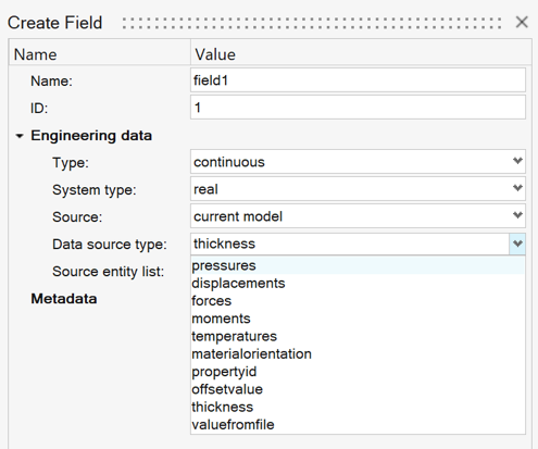 Figure 1.
 - CSV File
- The format for the .csv files depends on the system type and intended realization type:
-
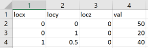
Figure 2. Scalar Data -
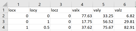
Figure 3. Vector Data -
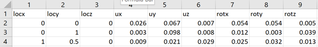
Figure 4. Displacement Data -
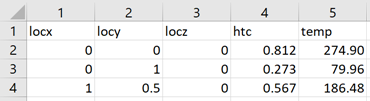
Figure 5. Convection Data -
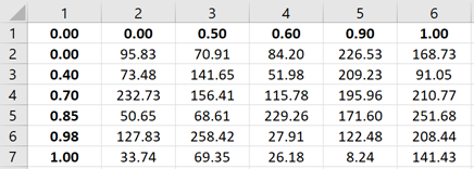
Figure 6. Parametric Data - HV Current Contour
- This option provides access to any results that are loaded and plotted in a neighboring HyperView window.
- Matrix
- A variety of model data can be used to generate fields via the Matrix Browser integration.
- Results
- Analysis output files can be used directly to create a field using this feature. All of the result formats supported in HyperView are supported for fields.
Realize Fields
-
In the Model Browser or Fields entity view , right-click on
a field and select Realize.
The Realize Fields dialog has multiple inputs and reconfigures depending on the type of realization.
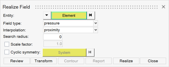
Figure 7.The first two inputs in this dialog define the “where” and “what” of the realization, and the remaining inputs specify the “how” with various mapping parameters.
-
Select a field realization type.
Depending on the field source data and whether the target is nodes or elements, different realization types are available to choose.
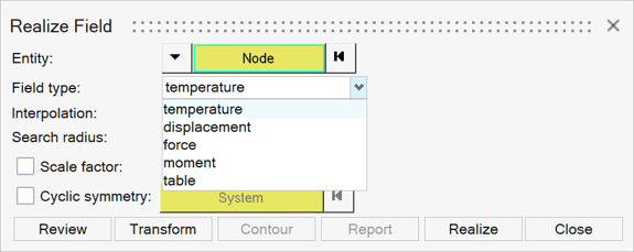
Figure 8.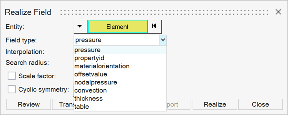
Figure 9.The listed realization types that are entities and attributes are self-explanatory, but there are also a couple of special types: convection and table.
- Convection
- In a convection realization, heat transfer coefficients and temperatures are mapped to the target elements. This option is only available for OptiStruct and Abaqus models, and requires a field sourced either from a convection data .csv file or from an AcuSolve results file.
- Table
- Also referred to as generic field mapping, with this feature the field data is mapped to the target entities, but the mapped values are just saved in a table rather than used to create or update FE entities. The table can then be used for various purposes, such as Matrix Browser based workflows.
-
Select a field mapping method, also known as an interpolation.
Several mapping methods are available depending on the field source data, target entities, and realization type.
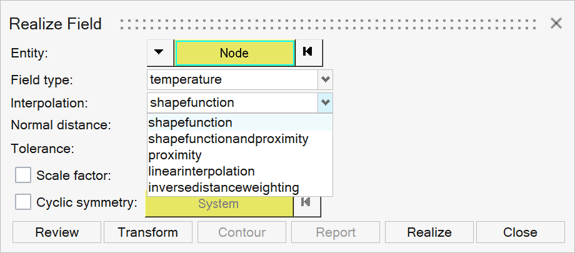
Figure 10.- Proximity
- This is the simplest mapping option. Target entities are assigned values based on the nearest source data point. Optionally, a maximum search radius may be specified with this method, in which case target entities are only assigned values if a source data point is found within that distance. If the radius is omitted (set to zero), values are assigned to all target entities based on the nearest source data point regardless of its distance.
- Inverse Distance Weighting
- With this method, the four source data points nearest to the target point are used to calculate a weighted average value using the formula below. Optionally, a maximum search radius can be specified, in which case only source data points within that radius are considered for each target point. The weighted average will proceed with less than four source values, but if no source points are within the specified radius of a target point, no value are assigned.
- Linear Interpolation
- With this method the target points (nodes or element centroids) are projected to the source mesh. The target value is calculated using a 3D linear interpolation based on the nodal values of the source element upon which the target point was projected. If a target point has no projection on the source mesh, the proximity method is attempted to find a value for that point. For fields created from .csv data, a source mesh is formed from the provided data points with Delaunay triangulation.
- Triangulation
- The triangulation method combines different aspects of some of the other algorithms. First, a triangular element is formed using the three source points nearest to the target point, and the target point is projected to the plane of the source element. The projected point must fall on the source element within the tolerance specified, and the projection must be less than the normal distance limit if it is specified. If the projection meets these criteria, the target value is calculated by shape function on the source element. Otherwise, a new source element is formed using the next nearest source data point, and a new projection is attempted. If a valid projection cannot be found using up to the 15 nearest source points, no target value are assigned.
- Shape Function
- True to its name, this method utilizes the element shape functions of the source mesh to calculate target values. For fields created from .csv data, a source mesh is formed from the provided data points with Delaunay triangulation. Each target point is projected to the nearest source element, determined based on the distance to the source element’s centroid. The projected point must fall on the source element within the tolerance specified, and the projection must be less than the normal distance limit if it is specified. If the projection meets these criteria, the target value is calculated by shape function on the source element. Otherwise, the next nearest source element is considered.
- Shape Function with Proximity
- This method first uses the shape function method as described above to assign values to all target points within an acceptable distance from the source mesh. Any target points that fall too far outside the source mesh are then assigned values using the proximity method.
- Force Balance
- This method is specifically designed to map a field of nodal forces, ensuring that the net forces on the target are equivalent to those on the source. OptiStruct is required for this method as it is used in the background.