ACU-T: 4102 Fluidized Bed using the Granular Multiphase Model
Prerequisites
This tutorial provides the instructions for setting up and running a gas-solid fluidized bed simulation using the granular multiphase model. Prior to starting this tutorial, you should have already run through the introductory tutorial, ACU-T: 1000 Basic Flow Set Up, and have a basic understanding of HyperWorks CFD and AcuSolve. To run this simulation, you will need access to a licensed version of HyperWorks CFD and AcuSolve.
Prior to running through this tutorial, click here to download the tutorial models. Extract ACU-T4102_FluidizedBed.hm from HyperWorksCFD_tutorial_inputs.zip.
Problem Description
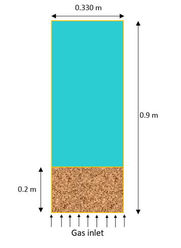
Figure 1.
| Phase | Density (kg/m3) | Viscosity (Pa s) |
|---|---|---|
| Gas | 21.56 | 1.781e-05 |
| Particle | 910 | - |
Start HyperWorks CFD and Open the HyperMesh Database
-
From the Home tools, Files tool group, click the Open Model tool.

Figure 2.The Open File dialog opens.
Validate the Geometry
The Validate tool scans through the entire model, performs checks on the surfaces and solids, and flags any defects in the geometry, such as free edges, closed shells, intersections, duplicates, and slivers.
Figure 3.
Set Up Flow
Set the General Simulation Parameters
-
From the Flow ribbon, click the Physics tool.

Figure 4.The Setup dialog opens. -
In the Material Library dialog, select Granular
Multiphase, switch to the My Material
tab, then click
 to add a new material.
-
Set the diameter, drag model, and other granular parameters as shown in the
image below.
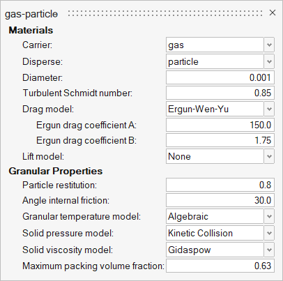
Figure 5. -
Set the gravity to 0, -9.81, 0 and the pressure scale to
Absolute.
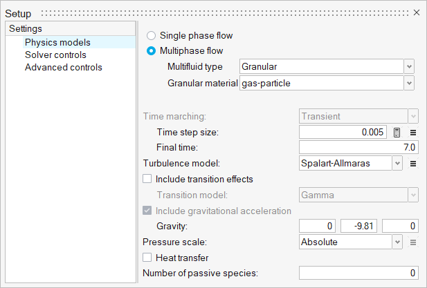
Figure 6. -
Click the Solver controls setting and set the Minimum
and Maximum stagger iterations to 2 and
4, respectively.
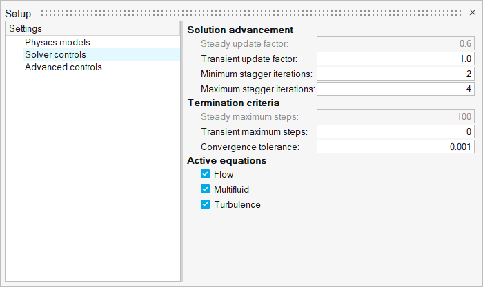
Figure 7.
Assign Material Properties
-
From the Flow ribbon, click the Material tool.

Figure 8. -
On the guide bar, click
 to exit
the tool.
to exit
the tool.
Define Flow Boundary Conditions
-
From the Flow ribbon, click the Constant tool.

Figure 9. -
Click the inlet face highlighted in the figure below.
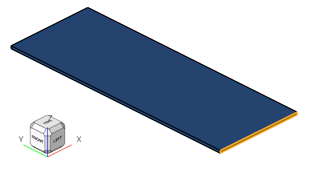
Figure 10. -
In the microdialog, enter the values shown in the figure below.
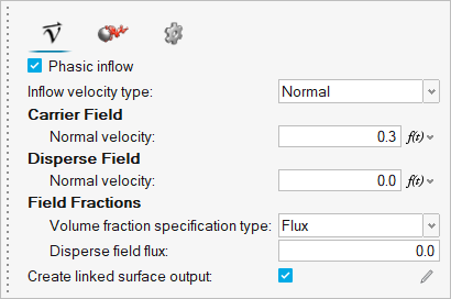
Figure 11. -
In the turbulence tab, set the turbulence input type to
Direct and set the eddy viscosity value to
0.0001.
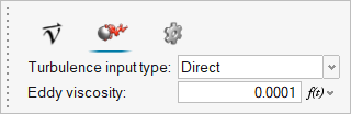
Figure 12. -
On the guide bar, click
 to execute
the command and exit the tool.
to execute
the command and exit the tool.
-
Click the Outlet tool.

Figure 13. -
Select the face highlighted below and verify the settings in the
microdialog.
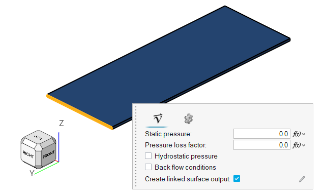
Figure 14. -
Click on the guide bar.
-
Click the Slip tool.

Figure 15. -
Select the top and bottom faces highlighted below then click on the
guide bar.
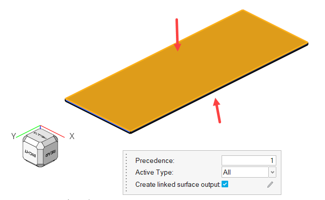
Figure 16.
Generate the Mesh
-
From the Mesh ribbon, click the
Volume tool.

Figure 17.Note: If the model has not been validated, you are prompted to create the simulation model before running the batch mesh. -
In the Meshing Operations dialog, check that the Average
Element size is set to 0.01.
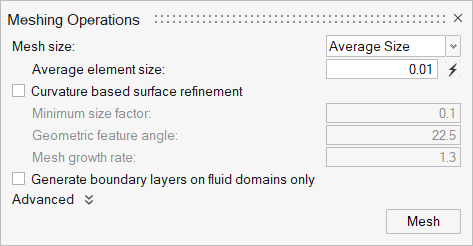
Figure 18.
Define Nodal Outputs
-
From the Solution ribbon, click the Field tool.

Figure 19.The Field Output dialog opens. -
Set the time interval to 10.
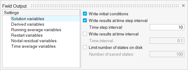
Figure 20.
Define the Nodal Initial Conditions
-
From the Solution ribbon, click the
Plane tool.

Figure 21. -
In the variable dialog, click in the top-left corner and select
Carrier Volume Fraction.
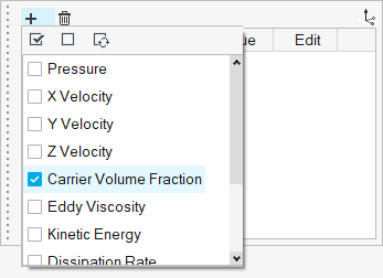
Figure 22. -
Click
 in the top-right corner of the dialog.
The Vector tool appears, which can be used change the location and orientation of the plane defining the initial condition.
in the top-right corner of the dialog.
The Vector tool appears, which can be used change the location and orientation of the plane defining the initial condition. -
In the Vector tool, verify that the orientation of the tool is along the
negative y-axis then click XYZ.
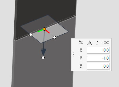
Figure 23. -
Enter the coordinates of the center of plane as shown in the figure
below.
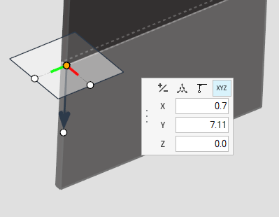
Figure 24. -
Click on the guide bar then save the model.
Run AcuSolve
-
From the Solution ribbon, click the Run tool.

Figure 25.The Launch AcuSolve dialog opens. -
Expand Default initial conditions, uncheck
Pre-compute flow, and set the velocity values to
0. Uncheck Pre-compute
Turbulence.
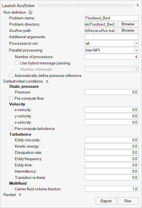
Figure 26.
Post-Process the Results with HW-CFD Post
-
Click the Boundary Groups tool.

Figure 27. -
Click
 and set the colormap properties as shown
below.
and set the colormap properties as shown
below.
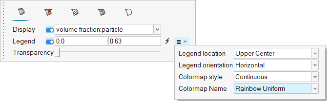
Figure 28. -
Click on the guide bar to create the volume fraction contour
plot.
-
Click the play icon at the bottom of the modeling window to play the animation.
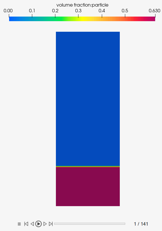
Figure 29.
Summary
In this tutorial, you learned how to set up and solve a fluidized bed simulation using the Granular multiphase model available in AcuSolve using HyperWorks CFD. You started by importing the HyperWorks CFD input database and then defined the flow setup. Once the solution was computed, you created a contour plot of particle volume fraction using HyperWorks CFD Post.