ACU-T: 4300 Species Transport Modeling
This tutorial provides instructions for modeling species transport using HyperWorks CFD. Prior to starting this tutorial, you should have already run through the introductory tutorial, ACU-T: 1000 Basic Flow Set Up, and have a basic understanding of HyperWorks CFD and AcuSolve. To run this simulation, you will need access to a licensed version of HyperWorks CFD and AcuSolve.
Prior to running through this tutorial, click here to download the tutorial models. Extract ACU-T4300_HoneyTeaSpecies.hm from HyperWorksCFD_tutorial_inputs.zip.
Problem Description
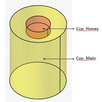
Figure 1.
Start HyperWorks CFD and Open the HyperMesh Database
-
From the Home tools, Files tool group, click the Open Model tool.

Figure 2.The Open File dialog opens.
Validate the Geometry
-
From the Geometry ribbon, click the Validate tool.

Figure 3.The Validate tool scans through the entire model, performs checks on the surfaces and solids, and flags any defects in the geometry, such as free edges, closed shells, intersections, duplicates, and slivers.The current model doesn’t have any of the issues mentioned above. Alternatively, if any issues are found, they are indicated by the number in the brackets adjacent to the tool name.
Observe that a blue check mark appears on the top-left corner of the Validate icon. This indicates that the tool found no issues with the geometry model.
Figure 4.
Set Up Flow
Set the General Simulation Parameters
-
From the Flow ribbon, click the Physics tool.

Figure 5.The Setup dialog opens. -
Under the Physics models setting:
- Set Time marching to Transient.
- Set the Time step size to 0.125.
- Select Laminar as the Turbulence model.
- Check the Include Gravitational Acceleration option and set the gravity to 9.81 m/s2 in the z direction.
- Set the Number of passive species to 1.
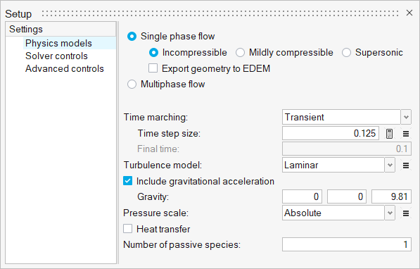
Figure 6. -
Click the Solver controls setting then set the Transient
maximum steps to 80.
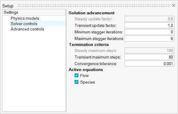
Figure 7.
Assign Material Properties
-
From the Flow ribbon, click the Material Library tool.

Figure 8.The Material Library dialog opens. -
Click
 to create a new material.
-
For density:
- Change the type to Piecewise Linear.
- Define the Curve fit variable as Species 1.
-
Click
 twice under Function then enter
1000 kg/m3 and
1500 kg/m3 in the Y column for the
density of water and honey, respectively.
twice under Function then enter
1000 kg/m3 and
1500 kg/m3 in the Y column for the
density of water and honey, respectively.
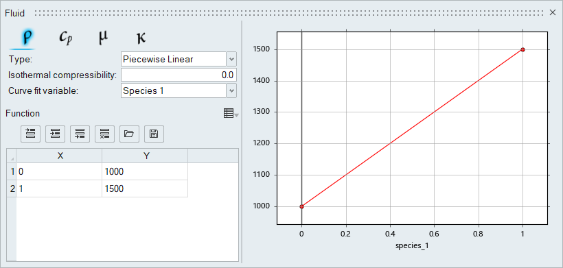
Figure 9. -
Similarly, define the viscosity values for water and honey according to the
figure below.
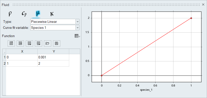
Figure 10. -
Close the material editing dialog, then rename the Fluid material to
Honey.
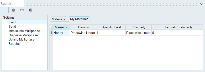
Figure 11. -
From the Flow ribbon, click the Material tool.

Figure 12. -
Select Honey from the Material drop-down menu.
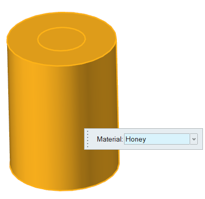
Figure 13. -
On the guide bar, click
 to execute
the command and exit the tool.
to execute
the command and exit the tool.
Define Flow Boundary Conditions
-
From the Flow ribbon, click the Slip tool.

Figure 14. -
Select the top two surfaces highlighted in the figure below then click
 on the
guide bar.
on the
guide bar.
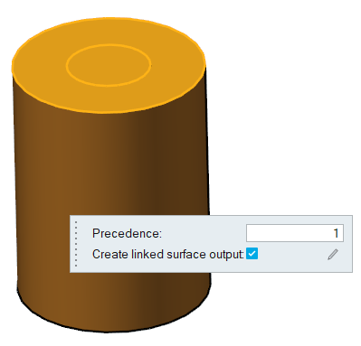
Figure 15.
Define Nodal Initial Conditions
-
From the Solution ribbon, click the Part tool.

Figure 16. -
Select the volume highlighted below.
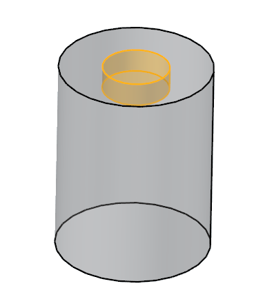
Figure 17. -
In the microdialog, click and
select Species 1 from the list.
-
Set the Type to Constant and the Value to
1.
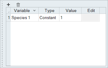
Figure 18.
Run AcuSolve
-
From the Solution ribbon, click the Run tool.

Figure 19.The Launch AcuSolve dialog opens. -
Leave the remaining options as default and click
Run to launch AcuSolve.
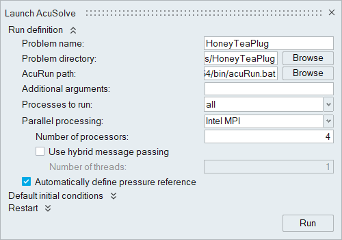
Figure 20.
Post-Process the Results with HW-CFD Post
-
Select the AcuSolve log file in your problem
directory to load the results for post-processing.
The solid and all the surfaces are loaded in the Post Browser.
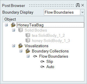
Figure 21. -
From the Post ribbon, click the Slice Planes tool.

Figure 22. -
Select the plane shown in the figure below.
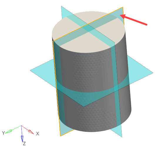
Figure 23. -
In the slice plane microdialog, click
 to
create the slice plane.
to
create the slice plane.
-
Activate the Legend radio button then click
 and set the Colormap name to
Rainbow Uniform.
and set the Colormap name to
Rainbow Uniform.
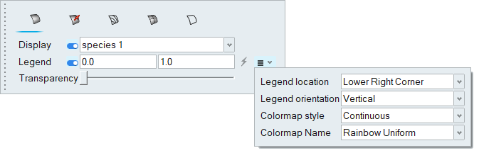
Figure 24. -
Click on the guide bar.
-
Make sure that the time scale at bottom of the modeling window is at 1 sec.

Figure 25. -
Adjust the time scale to show 2 sec, 4, sec, 6 sec, 8 sec, and 10 sec.
The distribution of species 1 (honey) at those times is shown below.
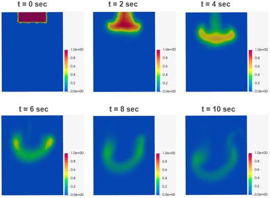
Figure 26. -
Click the Boundary Groups tool.

Figure 27. -
In the microdialog, move the Transparency slider to the
middle to add a transparency effect.
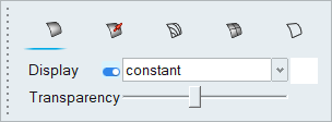
Figure 28. -
Click on the guide bar.
-
Click the Iso-Surfaces tool.

Figure 29. -
In the Iso-function microdialog, change the Iso
Variable to species 1 and set the Iso Value to
0.5
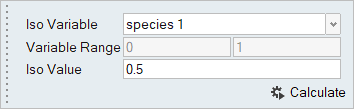
Figure 30. -
Click Calculate then click .
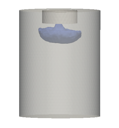
Figure 31. Distribution of species at 3 sec
Summary
In this tutorial, you successfully learned how to set up and solve a simulation involving species transport using HyperWorks CFD. You started by opening the HyperMesh input file with the geometry and then defined the simulation parameters, fluid material, and boundary conditions. Once the solution was computed, you visualized the results of species transport with help of planes and an iso-surface.