OS-T: 8030 Flutter Analysis of a General Transport Aircraft Model
This tutorial demonstrates the flutter analysis of an a General Transport Aircraft (GTA) model, using the KE method.
Preprocessing is done using Altair HyperWorks in the OptiStruct User profile. A model with existing structural and aeroelastic data is used as a base model and this tutorial demonstrates the creation of entities specific to flutter analysis.
Flutter is a dynamic instability in which the aerodynamic loads on a flexible body couple with its natural modes of vibration to produce oscillatory motions with increasing amplitude.
Using flutter analysis, the critical velocity to avoid flutter is identified for a given altitude. Once determined, designers aim to avoid their system nearing this critical velocity.
- Define flutter analysis using the KE method
- Define complex eigenvalue related entries
- Submit the job
- Post-process the results
Launch HyperWorks and Import the Model
Refer to Access the Model Files for more details about obtaining the tutorial model file. The model file required for this tutorial is aeroelasticity_flutter.fem
-
In the Solver Import Options dialog, for Reader select
OptiStruct.
The OptiStruct user profile loads. The functionality of HyperWorks is paired down to the appropriate template, macro menu, and import reader to create models in OptiStruct.
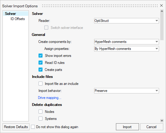
Figure 1. OptiStruct User Profile in HyperWorks -
Click Import.
The base model is loaded into HyperWorks.
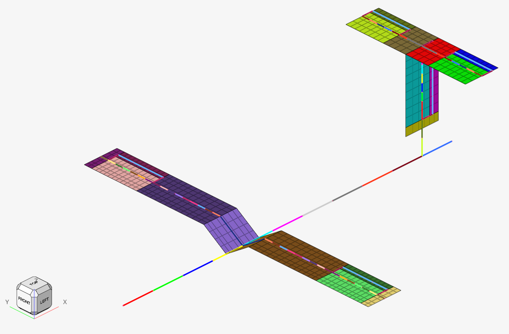
Figure 2. Base Model of Aircraft
Open the Aeroelasticity Browser
The Aeroelasticity Browser is useful for upcoming tasks in this tutorial.
-
On the Aeroelasticity ribbon, hover over any tool group
and click the satellite icon that appears.
The Aeroelasticity Browser opens.
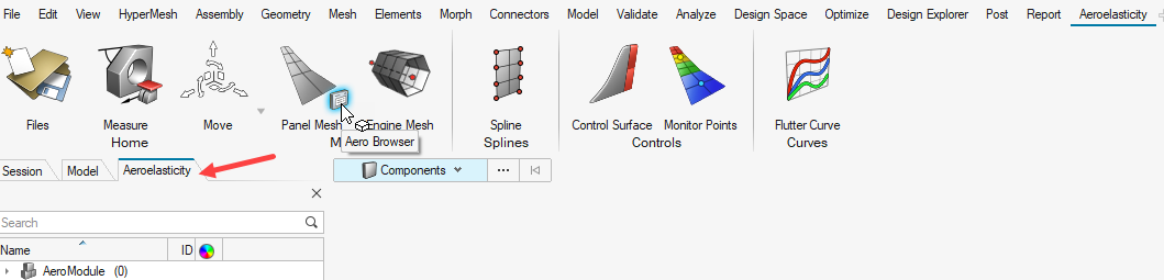
Figure 3. Access the Aeroelasticity Browser
Set Up the Model
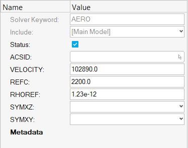
Create AERO Entry
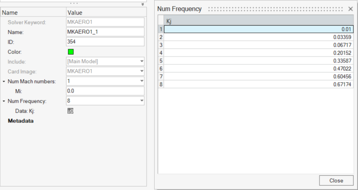
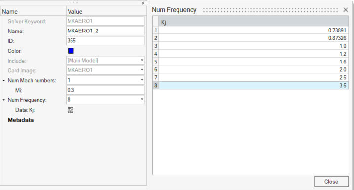
Create MKAERO1 Entries
In this step, the MKAERO1 entry is used to define the Mach number and reduced frequency table. Two MKAERO1 entries are created, since each MKAERO1 entry only allows a maximum of 8 fields.
These values, along with the reference density from the AERO entry are used to calculate the aerodynamic matrix.
Create FLFACT Entries
-
For FORMAT, select Factors from the drop-down
menu.
With this option, you can specify a list of aerodynamic factor values directly.
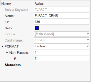
Figure 7. Definition of FLFACT Entry using IDS -
Create a third FLFACT entry.
-
Enter values in the browser as shown in Figure 8.
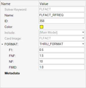
Figure 8. Definition of FLFACT Entry using THRU_FORMAT
-
Enter values in the browser as shown in Figure 8.
Create FLUTTER Entry
In this step, the FLUTTER entry is used to define the flutter analysis setup. The FLFACT entries defined in the previous step are also referenced in this FLUTTER entry.
-
Reference the previously created FLFACT entries.
-
For DENS, click and select
 .
.
- In the Advanced Selection dialog, choose the FLFACT entry you created for the density ratios and click OK.
- For MACH, select the FLFACT entry you created for the Mach numbers.
- For RFREQ, select the FLFACT entry you created for the reduced frequencies.
-
For DENS, click and select
-
For IMETH, select L from the drop-down menu.
This sets the interpolation method to linear.
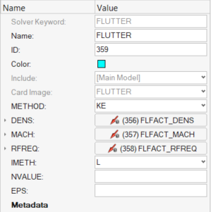
Figure 9. Definition of FLUTTER Entry
Create EIGRL Entry
In flutter analysis, OptiStruct uses the modal approach where the structural-vibration modes in a selected frequency range are used as the degrees of freedom. Hence, the EIGRL Bulk Data Entry is defined.
-
Enter the values as shown in Figure 10 to define the entry.
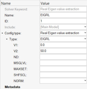
Figure 10. Definition of EIGRL Entry
Create PARM, VREF Entry
The output of flutter analysis can be postprocessed in the form of Velocity-Damping (V-g) and Velocity-Frequency (V-f) curves. PARAM, VREF can be used to convert the output velocities from flutter analysis to different unit systems.
This model is built in the units of mm, N, sec. The output velocity (in mm/sec) is converted to knots using this parameter.
Create Flutter Analysis Subcase
In this step, the previously created Bulk Data Entries are referenced in the Flutter Analysis subcase.
-
Reference the previously created Bulk Data Entries as shown in Figure 11.
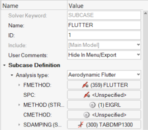
Figure 11. Subcase Definition for Flutter Analysis
Export the Input File
In this step, the input file is exported to the working directory. This file is later solved using OptiStruct as the solver.
Submit the Job
-
For Input file, use
 to browse your working directory for the desired
file.
to browse your working directory for the desired
file.
-
For Options, click
 .
.
- In the Select Solver Options dialog, click the -nt check box.
- Enter 8 for the argument.
- Click OK.
- Click the -out check box.
-
Click Run.
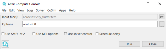
Figure 12. Altair Compute ConsoleIf the job is successful, the new results files should be in the working directory. If any errors are present, look in the aeroelasticity_flutter.out file for error messages that could help debug the input deck.
Post-Process the Results
Review Flutter Analysis Summary
The summary from flutter analysis is available by default in the .flt file. This ASCII file can be viewed in any text editor.
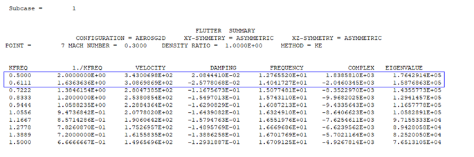
Figure 13. Flutter Analysis Summary from .flt File
By definition, instability (flutter or divergence) occurs when the damping values are zero.
At this point, if the frequency is zero, the instability is due to divergence.
Otherwise, the instability is due to flutter. In the scope of this tutorial (non-zero frequencies), determination of instability due to flutter is explained.
Determine Flutter Point from V-g and V-f Plots
The V-g and V-f plots are a more visual and robust way of post-processing. Among all the flutter points determined in the previous step, the flutter point corresponding to the lowest velocity is determined.
-
In the Aeroelasticity Browser, select the Flutter Curves
tool.
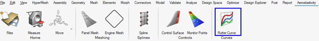
Figure 14. Access the Flutter Curves Tool -
Select Plot to plot the V-g curve.
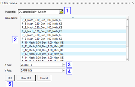
Figure 15. Steps to Plot the V-g Curve in the Flutter Curve Tool -
Determine the flutter points (where damping = 0).
-
Zoom in further on the plot to determine the velocity at this flutter
point is 327.668.
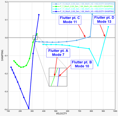
Figure 16. Identify the Flutter Points. The flutter point corresponding to the lowest velocity is visually identified.
-
Zoom in further on the plot to determine the velocity at this flutter
point is 327.668.
-
Select Plot to plot the V-f curve.
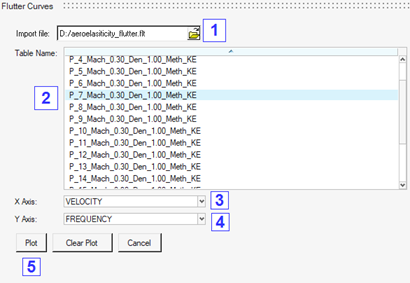
Figure 17. Steps to Plot the V-f Curve in the Flutter Tool -
Zoom in on the graph to determine the frequency value for the 7th mode at a
velocity of 327.688.
In this tutorial, the frequency value is 13.334.
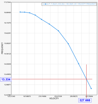
Figure 18. Identify Frequency Value at Critical Flutter Point from V-f CurveIn this way, the V-g and V-f plots are used to determine the lowest velocity at which flutter occurs. The frequency of the system is then determined. From the density ratio of the flutter mode, you can learn the altitude at which flutter instability occurs. You can then aim to keep the system from nearing this velocity and altitude.