Dynamic Aeroelastic Analysis

Dynamic Aeroelastic Analysis is the study of the deflection in flexible structures under aerodynamic loads, where the forces and acceleration are time dependent.

Flutter Analysis

Aeroelastic flutter is a dynamic instability of a structure associated with the interaction of aerodynamic, elastic, and inertial loads.

Flutter analysis of aeroelastic systems involves determining the velocity (and hence Mach Number) of the system and the frequency of oscillation at which the system attains the state of flutter. In this phenomenon, the aerodynamic loads on a flexible body couple with its natural modes of vibration to produce oscillatory motions with increasing amplitude.

This may lead to catastrophic structural failure. Therefore, structures exposed to aerodynamic loads must be carefully designed to avoid flutter.

In finite element analysis, the prediction of flutter involves a series of complex eigenvalue solutions. OptiStruct uses the modal approach where the structural-vibration modes in a selected frequency range are used as the degrees of freedom.

Methods

The four different methods for flutter analysis supported in OptiStruct are K, KE, PK and PKNL.

For each of these methods described below, the complex eigenvalues ( p MathType@MTEF@5@5@+= feaagKart1ev2aaatCvAUfeBSjuyZL2yd9gzLbvyNv2CaerbuLwBLn hiov2DGi1BTfMBaeXatLxBI9gBaerbd9wDYLwzYbItLDharqqtubsr 4rNCHbGeaGqiVu0Je9sqqrpepC0xbbL8F4rqqrFfpeea0xe9Lq=Jc9 vqaqpepm0xbba9pwe9Q8fs0=yqaqpepae9pg0FirpepeKkFr0xfr=x fr=xb9adbaqaaeGaciGaaiaabeqaamaabaabaaGcbaGaam4zaaaa@36E2@ ) are extracted for a particular case, from which the pairs of airspeed and damping ( V MathType@MTEF@5@5@+= feaagKart1ev2aaatCvAUfeBSjuyZL2yd9gzLbvyNv2CaerbuLwBLn hiov2DGi1BTfMBaeXatLxBI9gBaerbd9wDYLwzYbItLDharqqtubsr 4rNCHbGeaGqiVu0Je9sqqrpepC0xbbL8F4rqqrFfpeea0xe9Lq=Jc9 vqaqpepm0xbba9pwe9Q8fs0=yqaqpepae9pg0FirpepeKkFr0xfr=x fr=xb9adbaqaaeGaciGaaiaabeqaamaabaabaaGcbaGaamOvaaaa@36D1@ - p MathType@MTEF@5@5@+= feaagKart1ev2aaatCvAUfeBSjuyZL2yd9gzLbvyNv2CaerbuLwBLn hiov2DGi1BTfMBaeXatLxBI9gBaerbd9wDYLwzYbItLDharqqtubsr 4rNCHbGeaGqiVu0Je9sqqrpepC0xbbL8F4rqqrFfpeea0xe9Lq=Jc9 vqaqpepm0xbba9pwe9Q8fs0=yqaqpepae9pg0FirpepeKkFr0xfr=x fr=xb9adbaqaaeGaciGaaiaabeqaamaabaabaaGcbaGaam4zaaaa@36E2@ ), and airspeed and frequency ( V MathType@MTEF@5@5@+= feaagKart1ev2aaatCvAUfeBSjuyZL2yd9gzLbvyNv2CaerbuLwBLn hiov2DGi1BTfMBaeXatLxBI9gBaerbd9wDYLwzYbItLDharqqtubsr 4rNCHbGeaGqiVu0Je9sqqrpepC0xbbL8F4rqqrFfpeea0xe9Lq=Jc9 vqaqpepm0xbba9pwe9Q8fs0=yqaqpepae9pg0FirpepeKkFr0xfr=x fr=xb9adbaqaaeGaciGaaiaabeqaamaabaabaaGcbaGaamOvaaaa@36D1@ - f MathType@MTEF@5@5@+= feaagKart1ev2aaatCvAUfeBSjuyZL2yd9gzLbvyNv2CaerbuLwBLn hiov2DGi1BTfMBaeXatLxBI9gBaerbd9wDYLwzYbItLDharqqtubsr 4rNCHbGeaGqiVu0Je9sqqrpepC0xbbL8F4rqqrFfpeea0xe9Lq=Jc9 vqaqpepm0xbba9pwe9Q8fs0=yqaqpepae9pg0FirpepeKkFr0xfr=x fr=xb9adbaqaaeGaciGaaiaabeqaamaabaabaaGcbaGaam4zaaaa@36E2@ ) can be ascertained.

The precise form of eigenvalues differs for each of the methods.

For the K and KE methods, the eigenvalue is given by:(1)
p 2 = V 2 1 + i g MathType@MTEF@5@5@+= feaagKart1ev2aaatCvAUfeBSjuyZL2yd9gzLbvyNv2CaerbuLwBLn hiov2DGi1BTfMBaeXatLxBI9gBaerbd9wDYLwzYbItLDharqqtubsr 4rNCHbGeaGqiVu0Je9sqqrpepC0xbbL8F4rqqrFfpeea0xe9Lq=Jc9 vqaqpepm0xbba9pwe9Q8fs0=yqaqpepae9pg0FirpepeKkFr0xfr=x fr=xb9adbaqaaeGaciGaaiaabeqaamaabaabaaGcbaGaamiCamaaCa aaleqabaGaaGOmaaaakiabg2da9maalaaabaGaeyOeI0IaamOvamaa CaaaleqabaGaaGOmaaaaaOqaaiaaigdacqGHRaWkcaWGPbGaam4zaa aaaaa@3F26@
For PK and PKNL methods, the eigenvalue is given by:(2)
p = ω ( γ ± i ) MathType@MTEF@5@5@+= feaagKart1ev2aaatCvAUfeBSjuyZL2yd9gzLbvyNv2CaerbuLwBLn hiov2DGi1BTfMBaeXatLxBI9gBaerbd9wDYLwzYbItLDharqqtubsr 4rNCHbGeaGqiVu0Je9sqqrpepC0xbbL8F4rqqrFfpeea0xe9Lq=Jc9 vqaqpepm0xbba9pwe9Q8fs0=yqaqpepae9pg0FirpepeKkFr0xfr=x fr=xb9adbaqaaeGaciGaaiaabeqaamaabaabaaGcbaGaamiCaiabg2 da9iabeM8a3naabmaabaGaeq4SdCMaeyySaeRaamyAaaGaayjkaiaa wMcaaaaa@3FCA@
Where,
γ
Transient decay rate coefficient.
ω
Circular frequency, given by 2 π f MathType@MTEF@5@5@+= feaagKart1ev2aaatCvAUfeBSjuyZL2yd9gzLbvyNv2CaerbuLwBLn hiov2DGi1BTfMBaeXatLxBI9gBaerbd9wDYLwzYbItLDharqqtubsr 4rNCHbGeaGqiVu0Je9sqqrpepC0xbbL8F4rqqrFfpeea0xe9Lq=Jc9 vqaqpepm0xbba9pwe9Q8fs0=yqaqpepae9pg0FirpepeKkFr0xfr=x fr=xb9adbaqaaeGaciGaaiaabeqaamaabaabaaGcbaGaaGOmaiabec 8aWjaadAgaaaa@395A@ .
  • K Method:
    • The philosophy behind the K method is to inject the system with artificial damping (in the form of a structural damping term) to push the system to the flutter point.
    • A set of complex eigenvalues is output at every combination of density, Mach number, and reduced frequency from the FLFACT entries.
    • For this reason, the results obtained from the K method are slightly difficult to interpret.
  • KE Method:
    • The KE method is a variant of the K method with the following differences.
      • The viscous damping terms are ignored.
      • The complex modes are not output.
      • The flutter output is arranged based on modes and sorted using an eigenvalue extrapolation technique.
    • These features imply that the KE method is a computationally inexpensive and easy-to-interpret version of the K method.
  • PK Method:
    • The PK method allows for a general flutter analysis to be performed using doublet lattice aerodynamics (that assumes simple harmonic motion) using an iterative process.
    • In this method, the imaginary contributions to the stiffness matrix are ignored. This means that structural damping terms and modal damping with PARAM, KDAMP, -1 will not be taken into account.
    • The eigenvalue extraction is carried out for every combination of density, Mach number, and velocity from the FLFACT entries.
    • An initial guess of the reduced frequency ( k MathType@MTEF@5@5@+= feaagKart1ev2aaatCvAUfeBSjuyZL2yd9gzLbvyNv2CaerbuLwBLn hiov2DGi1BTfMBaeXatLxBI9gBaerbd9wDYLwzYbItLDharqqtubsr 4rNCHbGeaGqiVu0Je9sqqrpepC0xbbL8F4rqqrFfpeea0xe9Lq=Jc9 vqaqpepm0xbba9pwe9Q8fs0=yqaqpepae9pg0FirpepeKkFr0xfr=x fr=xb9adbaqaaeGaciGaaiaabeqaamaabaabaaGcbaGaam4zaaaa@36E2@ ) is used to solve the complex eigen problem whose output returns an updated reduced frequency; the process being repeated until convergence. Modes are tracked across airspeeds using the left and right complex eigenvectors.
  • PKNL Method:
    • The PKNL method is a variant of the PK method designed with ‘no looping’.
    • In this method, the number of entries in the FLFACT data for density ratios, Mach numbers, and velocities need to be the same and the eigenvalue extraction is carried out at each linear selection of density ratio, Mach number, and velocity.
The following scenarios outlines the difference between the PK and PKNL methods:
  • Scenario 1:
    The flutter analysis is carried out at the following points: (0.5, 0.3, 100), (0.5, 0.3, 200), (1.0, 0.3, 100), (1.0, 0.3, 200), (0.5, 0.4, 100), (0.5, 0.4, 200), (1.0, 0.4, 100) and (1.0, 0.4, 200).
    $--1---><---2--><---3--><---4--><--5---><--6---><---7--><--8---><---9-->
    FLUTTER      103      PK       1       2       3       L       4
    FLFACT         1     0.5     1.0
    FLFACT         2     0.3     0.4
    FLFACT         3   100.0   200.0
  • Scenario 2:
    The flutter analysis is carried out at the following points: (0.5, 0.3, 100) and (1.0, 0.4, 200).
    $--1---><---2--><---3--><---4--><--5---><--6---><---7--><--8---><---9-->
    FLUTTER      103    PKNL       1       2       3       L       4
    FLFACT         1     0.5     1.0
    FLFACT         2     0.3     0.4
    FLFACT         3   100.0   200.0

Input

Figure 1 summarizes the workflow of an aeroelastic flutter analysis in OptiStruct.


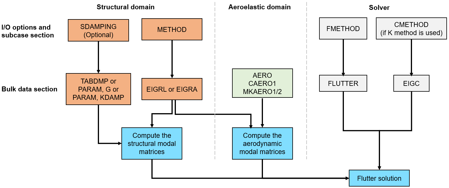
Figure 1. Flutter analysis workflow
The following tables summarize the relevant input file entries in an aeroelastic flutter analysis.
Table 1. Bulk Data Entries
Entry Description
AERO Defines flight conditions.
MKAERO1/MKAERO2 Specifies the Mach number and reduced frequency pairs for the explicit computation of the aerodynamic matrix.
FLFACT Specifies the values of flutter parameters (Density ratios, velocities, and reduced frequencies) for flutter analysis.
FLUTTER Selects the method (K/KE/PK/PKNL) and parameters for flutter analysis. This entry also references the definitions of FLFACT.
EIGC Selects the complex eigenvalue method for the K method.
EIGRL/EIGRA
  • Selects how the structural modes are computed and the number of them.
  • The number of structural modes can be changed with LMODES/LFREQ/HFREQ.
  • NVALUE in FLUTTER entry can be used to limit the number of eigenvalues printed in the .flt file.
PARAM, VREF Used to scale the output velocity: Vout = V/Vref.
DMI Defines real matrix data blocks.
Table 2. I/O Options and Subcase Information Entries
Entry Description
FMETHOD References the FLUTTER entry.
CMETHOD References the EIGC entry, for complex eigenvalue extraction (K method only).

Problem Setup

The following content of an input file gives an example of a typical aeroelastic flutter analysis setup.
$ ************************************************************
$ SNIPPET OF AN INPUT FILE FOR AEROELASTIC FLUTTER ANALYSIS
$ ************************************************************
SUBCASE 101
   SPC = 101
   METHOD = 102 
   FMETHOD = 103
   CMETHOD = 104 
BEGIN BULK
$--1---><--2---><--3---><--4---><--5---><--6---><--7---><--8---><--9---><--10-->
EIGRL   1       0.0     100.    4                               MASS
EIGC    109              
FLUTTER 103     K       1       2       3       L       4

FLFACT  1       0.1
FLFACT  2       .90
FLFACT  3       0.001   0.18    0.26    0.34    0.6 
AERO            102890. 2200.   .123E-110       0
MKAERO1 0.3                                                             +
+       0.01000 0.03359 0.06717 0.20152 0.33587 0.47022 0.60456 0.67174

$ other aeroelastic and structural entries

Output

The roots of the complex eigenvalue analysis are printed in the .flt file. A typical flutter analysis summary in the .flt file is shown below.


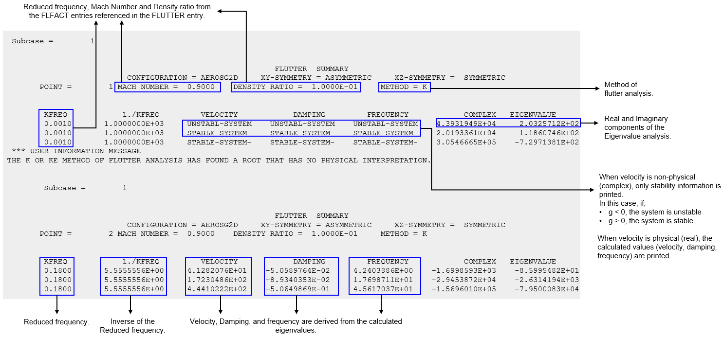
Figure 2. Flutter analysis summary in an example .flt file
For the K and KE methods:
  • The eigenvalue ( p MathType@MTEF@5@5@+= feaagKart1ev2aaatCvAUfeBSjuyZL2yd9gzLbvyNv2CaerbuLwBLn hiov2DGi1BTfMBaeXatLxBI9gBaerbd9wDYLwzYbItLDharqqtubsr 4rNCHbGeaGqiVu0Je9sqqrpepC0xbbL8F4rqqrFfpeea0xe9Lq=Jc9 vqaqpepm0xbba9pwe9Q8fs0=yqaqpepae9pg0FirpepeKkFr0xfr=x fr=xb9adbaqaaeGaciGaaiaabeqaamaabaabaaGcbaGaam4zaaaa@36E2@ ) is used to determine airspeed ( V MathType@MTEF@5@5@+= feaagKart1ev2aaatCvAUfeBSjuyZL2yd9gzLbvyNv2CaerbuLwBLn hiov2DGi1BTfMBaeXatLxBI9gBaerbd9wDYLwzYbItLDharqqtubsr 4rNCHbGeaGqiVu0Je9sqqrpepC0xbbL8F4rqqrFfpeea0xe9Lq=Jc9 vqaqpepm0xbba9pwe9Q8fs0=yqaqpepae9pg0FirpepeKkFr0xfr=x fr=xb9adbaqaaeGaciGaaiaabeqaamaabaabaaGcbaGaamOvaaaa@36D1@ ) and damping ( g MathType@MTEF@5@5@+= feaagKart1ev2aaatCvAUfeBSjuyZL2yd9gzLbvyNv2CaerbuLwBLn hiov2DGi1BTfMBaeXatLxBI9gBaerbd9wDYLwzYbItLDharqqtubsr 4rNCHbGeaGqiVu0Je9sqqrpepC0xbbL8F4rqqrFfpeea0xe9Lq=Jc9 vqaqpepm0xbba9pwe9Q8fs0=yqaqpepae9pg0FirpepeKkFr0xfr=x fr=xb9adbaqaaeGaciGaaiaabeqaamaabaabaaGcbaGaam4zaaaa@36E2@ ) using Equation 1.
    Note: This equation can be split into two equations for real and imaginary components and the two unknowns can be solved.
  • When the values of p MathType@MTEF@5@5@+= feaagKart1ev2aaatCvAUfeBSjuyZL2yd9gzLbvyNv2CaerbuLwBLn hiov2DGi1BTfMBaeXatLxBI9gBaerbd9wDYLwzYbItLDharqqtubsr 4rNCHbGeaGqiVu0Je9sqqrpepC0xbbL8F4rqqrFfpeea0xe9Lq=Jc9 vqaqpepm0xbba9pwe9Q8fs0=yqaqpepae9pg0FirpepeKkFr0xfr=x fr=xb9adbaqaaeGaciGaaiaabeqaamaabaabaaGcbaGaam4zaaaa@36E2@ are such that V MathType@MTEF@5@5@+= feaagKart1ev2aaatCvAUfeBSjuyZL2yd9gzLbvyNv2CaerbuLwBLn hiov2DGi1BTfMBaeXatLxBI9gBaerbd9wDYLwzYbItLDharqqtubsr 4rNCHbGeaGqiVu0Je9sqqrpepC0xbbL8F4rqqrFfpeea0xe9Lq=Jc9 vqaqpepm0xbba9pwe9Q8fs0=yqaqpepae9pg0FirpepeKkFr0xfr=x fr=xb9adbaqaaeGaciGaaiaabeqaamaabaabaaGcbaGaamOvaaaa@36D1@ is physical (real), the calculated values of velocity, damping and frequency are printed.
  • When the values of p MathType@MTEF@5@5@+= feaagKart1ev2aaatCvAUfeBSjuyZL2yd9gzLbvyNv2CaerbuLwBLn hiov2DGi1BTfMBaeXatLxBI9gBaerbd9wDYLwzYbItLDharqqtubsr 4rNCHbGeaGqiVu0Je9sqqrpepC0xbbL8F4rqqrFfpeea0xe9Lq=Jc9 vqaqpepm0xbba9pwe9Q8fs0=yqaqpepae9pg0FirpepeKkFr0xfr=x fr=xb9adbaqaaeGaciGaaiaabeqaamaabaabaaGcbaGaam4zaaaa@36E2@ are such that V MathType@MTEF@5@5@+= feaagKart1ev2aaatCvAUfeBSjuyZL2yd9gzLbvyNv2CaerbuLwBLn hiov2DGi1BTfMBaeXatLxBI9gBaerbd9wDYLwzYbItLDharqqtubsr 4rNCHbGeaGqiVu0Je9sqqrpepC0xbbL8F4rqqrFfpeea0xe9Lq=Jc9 vqaqpepm0xbba9pwe9Q8fs0=yqaqpepae9pg0FirpepeKkFr0xfr=x fr=xb9adbaqaaeGaciGaaiaabeqaamaabaabaaGcbaGaamOvaaaa@36D1@ is non-physical (complex), only stability information is printed for velocity, damping, and frequency values.
  • In such cases, when
    g < 0
    the system is unstable
    g > 0
    the system is stable
  • The determined values of V MathType@MTEF@5@5@+= feaagKart1ev2aaatCvAUfeBSjuyZL2yd9gzLbvyNv2CaerbuLwBLn hiov2DGi1BTfMBaeXatLxBI9gBaerbd9wDYLwzYbItLDharqqtubsr 4rNCHbGeaGqiVu0Je9sqqrpepC0xbbL8F4rqqrFfpeea0xe9Lq=Jc9 vqaqpepm0xbba9pwe9Q8fs0=yqaqpepae9pg0FirpepeKkFr0xfr=x fr=xb9adbaqaaeGaciGaaiaabeqaamaabaabaaGcbaGaamOvaaaa@36D1@ in conjunction with the user-specified reduced frequency ( k MathType@MTEF@5@5@+= feaagKart1ev2aaatCvAUfeBSjuyZL2yd9gzLbvyNv2CaerbuLwBLn hiov2DGi1BTfMBaeXatLxBI9gBaerbd9wDYLwzYbItLDharqqtubsr 4rNCHbGeaGqiVu0Je9sqqrpepC0xbbL8F4rqqrFfpeea0xe9Lq=Jc9 vqaqpepm0xbba9pwe9Q8fs0=yqaqpepae9pg0FirpepeKkFr0xfr=x fr=xb9adbaqaaeGaciGaaiaabeqaamaabaabaaGcbaGaam4zaaaa@36E2@ ) and reference chord length (REFC from AERO entry) can be used to calculate the frequency ( f MathType@MTEF@5@5@+= feaagKart1ev2aaatCvAUfeBSjuyZL2yd9gzLbvyNv2CaerbuLwBLn hiov2DGi1BTfMBaeXatLxBI9gBaerbd9wDYLwzYbItLDharqqtubsr 4rNCHbGeaGqiVu0Je9sqqrpepC0xbbL8F4rqqrFfpeea0xe9Lq=Jc9 vqaqpepm0xbba9pwe9Q8fs0=yqaqpepae9pg0FirpepeKkFr0xfr=x fr=xb9adbaqaaeGaciGaaiaabeqaamaabaabaaGcbaGaam4zaaaa@36E2@ ), (3)
    k = ω R E F C 2 V MathType@MTEF@5@5@+= feaagKart1ev2aaatCvAUfeBSjuyZL2yd9gzLbvyNv2CaerbuLwBLn hiov2DGi1BTfMBaeXatLxBI9gBaerbd9wDYLwzYbItLDharqqtubsr 4rNCHbGeaGqiVu0Je9sqqrpepC0xbbL8F4rqqrFfpeea0xe9Lq=Jc9 vqaqpepm0xbba9pwe9Q8fs0=yqaqpepae9pg0FirpepeKkFr0xfr=x fr=xb9adbaqaaeGaciGaaiaabeqaamaabaabaaGcbaGaam4Aaiabg2 da9maalaaabaGaeqyYdCNaamOuaiaadweacaWGgbGaam4qaaqaaiaa ikdacaWGwbaaaaaa@3E94@
    Using the calculated ω from Equation 3, (4)
    f = ω 2 π MathType@MTEF@5@5@+= feaagKart1ev2aaatCvAUfeBSjuyZL2yd9gzLbvyNv2CaerbuLwBLn hiov2DGi1BTfMBaeXatLxBI9gBaerbd9wDYLwzYbItLDharqqtubsr 4rNCHbGeaGqiVu0Je9sqqrpepC0xbbL8F4rqqrFfpeea0xe9Lq=Jc9 vqaqpepm0xbba9pwe9Q8fs0=yqaqpepae9pg0FirpepeKkFr0xfr=x fr=xb9adbaqaaeGaciGaaiaabeqaamaabaabaaGcbaGaamOzaiabg2 da9maalaaabaGaeqyYdChabaGaaGOmaiabec8aWbaaaaa@3C3D@
  • Since the KE method arranges the flutter summary by mode, the flutter point can be easily ascertained from a visual inspection of when the damping switches signs.
For the PK and PKNL methods:
  • The frequency ( f MathType@MTEF@5@5@+= feaagKart1ev2aaatCvAUfeBSjuyZL2yd9gzLbvyNv2CaerbuLwBLn hiov2DGi1BTfMBaeXatLxBI9gBaerbd9wDYLwzYbItLDharqqtubsr 4rNCHbGeaGqiVu0Je9sqqrpepC0xbbL8F4rqqrFfpeea0xe9Lq=Jc9 vqaqpepm0xbba9pwe9Q8fs0=yqaqpepae9pg0FirpepeKkFr0xfr=x fr=xb9adbaqaaeGaciGaaiaabeqaamaabaabaaGcbaGaam4zaaaa@36E2@ ) and damping ( g MathType@MTEF@5@5@+= feaagKart1ev2aaatCvAUfeBSjuyZL2yd9gzLbvyNv2CaerbuLwBLn hiov2DGi1BTfMBaeXatLxBI9gBaerbd9wDYLwzYbItLDharqqtubsr 4rNCHbGeaGqiVu0Je9sqqrpepC0xbbL8F4rqqrFfpeea0xe9Lq=Jc9 vqaqpepm0xbba9pwe9Q8fs0=yqaqpepae9pg0FirpepeKkFr0xfr=x fr=xb9adbaqaaeGaciGaaiaabeqaamaabaabaaGcbaGaam4zaaaa@36E2@ ) are extracted from the form of the eigen value using Equation 2.
    Note: This equation can be split into two equations for real and imaginary components and the two unknowns can be solved.

    The damping reported is:

    (5)
    g = 2 γ MathType@MTEF@5@5@+= feaagKart1ev2aaatCvAUfeBSjuyZL2yd9gzLbvyNv2CaerbuLwBLn hiov2DGi1BTfMBaeXatLxBI9gBaerbd9wDYLwzYbItLDharqqtubsr 4rNCHbGeaGqiVu0Je9sqqrpepC0xbbL8F4rqqrFfpeea0xe9Lq=Jc9 vqaqpepm0xbba9pwe9Q8fs0=yqaqpepae9pg0FirpepeKkFr0xfr=x fr=xb9adbaqaaeGaciGaaiaabeqaamaabaabaaGcbaGaam4zaiabg2 da9iaaikdacqaHZoWzaaa@3A4B@
  • In the case of purely real roots, the damping is:(6)
    g= 2pREFC ln( 2 )V MathType@MTEF@5@5@+= feaagKart1ev2aaatCvAUfeBSjuyZL2yd9gzLbvyNv2CaerbuLwBLn hiov2DGi1BTfMBaeXatLxBI9gBaerbd9wDYLwzYbItLDharqqtubsr 4rNCHbGeaGqiVu0Je9sqqrpepC0xbbL8F4rqqrFfpeea0xe9Lq=Jc9 vqaqpepm0xbba9pwe9Q8fs0=yqaqpepae9pg0FirpepeKkFr0xfr=x fr=xb9adbaqaaeGaciGaaiaabeqaamaabaabaaGcbaGaam4zaiabg2 da9maalaaabaGaaGOmaiaadchacaWGsbGaamyraiaadAeacaWGdbaa baGaciiBaiaac6gadaqadaqaaiaaikdaaiaawIcacaGLPaaacaWGwb aaaaaa@41E1@

The .flt file can be loaded into the “Flutter Curves” functionality of the aeroelasticity module of HyperWorks to easily generate the ( V MathType@MTEF@5@5@+= feaagKart1ev2aaatCvAUfeBSjuyZL2yd9gzLbvyNv2CaerbuLwBLn hiov2DGi1BTfMBaeXatLxBI9gBaerbd9wDYLwzYbItLDharqqtubsr 4rNCHbGeaGqiVu0Je9sqqrpepC0xbbL8F4rqqrFfpeea0xe9Lq=Jc9 vqaqpepm0xbba9pwe9Q8fs0=yqaqpepae9pg0FirpepeKkFr0xfr=x fr=xb9adbaqaaeGaciGaaiaabeqaamaabaabaaGcbaGaamOvaaaa@36D1@ - g MathType@MTEF@5@5@+= feaagKart1ev2aaatCvAUfeBSjuyZL2yd9gzLbvyNv2CaerbuLwBLn hiov2DGi1BTfMBaeXatLxBI9gBaerbd9wDYLwzYbItLDharqqtubsr 4rNCHbGeaGqiVu0Je9sqqrpepC0xbbL8F4rqqrFfpeea0xe9Lq=Jc9 vqaqpepm0xbba9pwe9Q8fs0=yqaqpepae9pg0FirpepeKkFr0xfr=x fr=xb9adbaqaaeGaciGaaiaabeqaamaabaabaaGcbaGaam4zaaaa@36E2@ ) and ( V MathType@MTEF@5@5@+= feaagKart1ev2aaatCvAUfeBSjuyZL2yd9gzLbvyNv2CaerbuLwBLn hiov2DGi1BTfMBaeXatLxBI9gBaerbd9wDYLwzYbItLDharqqtubsr 4rNCHbGeaGqiVu0Je9sqqrpepC0xbbL8F4rqqrFfpeea0xe9Lq=Jc9 vqaqpepm0xbba9pwe9Q8fs0=yqaqpepae9pg0FirpepeKkFr0xfr=x fr=xb9adbaqaaeGaciGaaiaabeqaamaabaabaaGcbaGaamOvaaaa@36D1@ - f MathType@MTEF@5@5@+= feaagKart1ev2aaatCvAUfeBSjuyZL2yd9gzLbvyNv2CaerbuLwBLn hiov2DGi1BTfMBaeXatLxBI9gBaerbd9wDYLwzYbItLDharqqtubsr 4rNCHbGeaGqiVu0Je9sqqrpepC0xbbL8F4rqqrFfpeea0xe9Lq=Jc9 vqaqpepm0xbba9pwe9Q8fs0=yqaqpepae9pg0FirpepeKkFr0xfr=x fr=xb9adbaqaaeGaciGaaiaabeqaamaabaabaaGcbaGaam4zaaaa@36E2@ ) curves without the use of any external post-processing tool.

Flutter Analysis Output

Currently, only the following output requests are supported with flutter analysis. Refer to Results Output by OptiStruct for supported output formats.
The following table summarizes information on the eigenvector output for different methods.
Method Comments
K Method
  • Eigenvector output is available in the form of points; each point corresponds to a reduced frequency.
  • At a given point, the results are available for each mode.
KE Method
  • Eigenvector output is not supported.
  • .h3d output file is not available.
PK/PKNL Method
  • Eigenvector output is available in the form of points; each point corresponds to a mode number.
  • Output is not available for the positive velocities in the FLFACT entry for velocity.
  • If output is desired for certain velocities, these velocities can be negated in the FLFACT entry.
  • This is only a convention; a negative velocity has no physical meaning. A positive value is always used for calculations regardless of the sign of velocity in the FLFACT entry.