Electrical Analysis
An electrical analysis involves calculation of electric potential in structures subject to electrical loads.
- Electrical conduction matrix
- Electric potential
- Electric current
This is the equilibrium equation of electric currents and is solved for the unknown electric potential.
Electrical Analysis in OptiStruct
- Steady State Electrical Conduction (SSEC)
- The loading (current or enforced voltage) is time independent.
- Multi Steady Electrical Conduction (MSEC)
- The loading (current or enforced voltage) is time dependent.
Coupled Electrical Analysis
Electrical analysis can be coupled with heat transfer analysis.
- Steady-State (linear/nonlinear) Heat Transfer analysis can only be coupled with SSEC.
- Transient (linear/nonlinear) Heat Transfer analysis can only be coupled
with MSEC.Note: Transient (linear/nonlinear) Heat Transfer analysis can still call an SSEC subcase via a DLOAD (that refers to a TLOAD, referencing a SSEC subcase). This is not a coupling and the solution from SSEC is used as a loading, like QVOL, in this case.
For an example use case, if the electrical load is constant and the electrical material is temperature independent, this method can greatly reduce computational time. Without this method, the solution must be computed at each time-step.
1-Way Coupling
- Example 1: Steady-State Heat Transfer Analysis Calls SSEC as Loading
-
Subcase 101 ANALYSIS ELEC SPC = 20 LOAD = 22 Subcase 102 ANALYSIS HEAT SPC = 21 JOULE = 101 LOAD = 25 - Example 2: SSEC Uses Steady-State Heat Transfer Analysis to Update Material
-
SUBCASE 101 ANALYSIS ELEC SPC = 20 LOAD = 22 TEMP(MAT) = 102 SUBCASE 102 ANALYSIS HEAT SPC = 21 LOAD = 25 - Example 3: Transient Heat Transfer Analysis Calls MSEC as Loading
-
SUBCASE 101
   ANALYSIS ELEC
   SPC = 20
   DLOAD = 23
SUBCASE 2
   ANALYSIS HEAT
   SPC  = 21
   DLOAD = 26
   TSTEP  = 9
BEGIN BULK
TLOAD1, 26, 101, ,JOULE, 28
TABLEG,28,
+,…
2-Way Coupling
- SSEC Uses Steady-State Heat Transfer to Update Material
- Joule heating from SSEC is applied to steady-state heat transfer analysis.
- MSEC Uses Transient Heat Transfer Analysis to Update Material
- Joule heating from MSEC is applied to transient heat transfer analysis.
Examples for 1-way and 2-way coupling can be extended to nonlinear steady-state heat transfer subcases.
Input
A summary of the relevant input file entries in an electrical analysis.
| Entry | Purpose |
|---|---|
| SPC, SPCD | Potential |
| CURRENT | Nodal current |
| CDENST4 | Current density |
| MAT1EC | Isotropic electrical material |
| MAT2EC | Anisotropic electrical material |
| MATT1EC, MATT2EC | Temperature dependent material |
| PGAP | Electrical resistance properties for gap elements |
| PCONTEC | Contact Electric Coefficient (CEC) for CONTACT element |
The TLOAD entry supports Joule loss density excitation (TYPE = J, JO, JOU, or JOUL). EXCITEID refers to the ID of a steady state electrical subcase from which the Joule loss density can be applied to a transient heat transfer subcase.
Analogy
The following table summarizes the analogy of some electrical analysis entries with the existing thermal/structural analysis.
| Type | Electrical Analysis | Thermal Analysis | Structural Analysis |
|---|---|---|---|
| Result output | Electrical potential | Temperature | Displacement |
| Electrical field | Temperature Gradient | Strain | |
| Loads and boundary conditions | CURRENT | FORCE | |
| CDENST4 | QBDY1 | PLOAD4 | |
| SPC (Electrical potential) | SPC (Temperature) | SPC (Displacement) | |
| SPCD (Electrical potential) | SPCD (Temperature) | SPCD (Displacement) | |
| Material | MAT1EC | MAT4 | MAT1 |
| MAT2EC | MAT5 | MAT9 | |
| MATT1EC | MATT4 | MATT1 | |
| MATT2EC | MATT5 | MATT9 |
Problem Setup
Example of an electrical analysis setup.
$ *************************************************************
$ EXAMPLE TO DEMONSTRATE AN ELECTRICAL ANALYSIS SETUP
$ *************************************************************
OLOAD     = 11
VOLTAGE   = 11
GPCURRENT = 11
ELECMAT   = 22
ELECFIELD = 22
HEAT      = 22
CURRDEN   = 22

SUBCASE        1
  LABEL HEAT
  ANALYSIS HEAT
  IC =        1
  JOULE =     2
  TSTEP =     9
  DLOAD =     28
  SPC   =     12
  NLPARM =    6

SUBCASE        2
  LABEL ELEC
  ANALYSIS ELEC
  DLOAD   =   3
  SPC     =  10
  TEMP(MAT) = 1.

BEGIN BULK
...
Example
A visual example of modeling Joule heating in a Busbar system.
Busbars are commonly used in many applications to provide power to various electronic boxes.
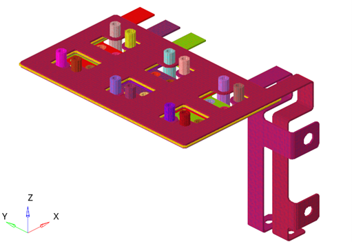
Figure 1. Busbar Model
An initial temperature of 20 degrees Celsius is applied to all the bodies.
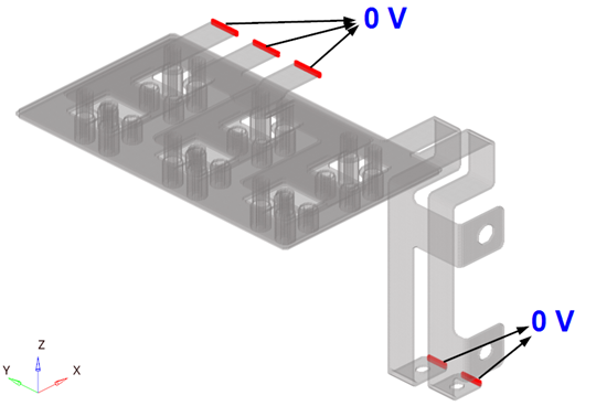
Figure 2. Boundary Conditions on Busbar Model. Zero potential is applied as shown in red
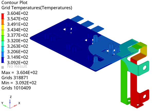
Figure 3. Temperature Distribution on Busbar
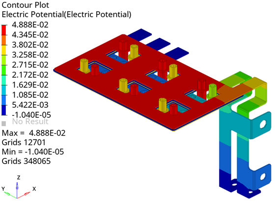
Figure 4. Electric Potential on Busbar
Output
Supported output requests for electrical analysis.
Currently, results are only available in .h3d format in a separate *_elecht.h3d file.
| Result | Purpose | Details |
|---|---|---|
| VOLTAGE | Voltage | Available by default |
| HEAT | Joule loss density | Available by default |
| CURRDEN | Current density | Available by default |
| ELECFIELD | Electric field | |
| ELECMAT | Conductivity and resistivity | |
| GPCURRENT | Gap current | |
| OLOAD | Applied nodal current |
A current balance summary table is available in the .out file for steady state electrical conduction analysis. This is similar to the SPCFORCE output table and consists of total applied current and SPC current.
This table is currently unavailable for MSEC analysis.