Contact
Contact is an integral aspect of the analysis and optimization techniques that is utilized to understand, model, predict, and optimize the behavior of physical structures and processes.
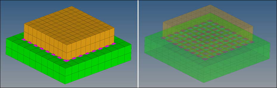
Figure 1.
The OptiStruct contact algorithm automatically handles these cases and a variety of options are available to control the contact interface definition. The CONTACT and TIE Bulk Data Entries in conjunction with the PCONT Bulk Data Entry (if required) can be used to typically set up the majority of contact solutions in OptiStruct. The various CONTPRM parameters can be utilized to modify and control the contact parameters. The SUPORT-based Fast Contact solution requires setting up SUPORT entries (optionally, user-defined MPCs, SPCs, and SPOINTs) to generate the contact.
Contact Discretization
Contact between the main and secondary surfaces can be constructed through three main approaches. This process is called discretization, and it defines the basic structure of the contact elements that are constructed to handle the contact condition.
Node-to-Surface Discretization
The Node-to-Surface Discretization approach involves the creation of contact elements linking the Main Surfaces to Secondary Nodes.

Figure 2.

- One secondary node

- A few main nodes

- One main face including the main nodes

- One projection from the secondary node to the main face

Figure 3.
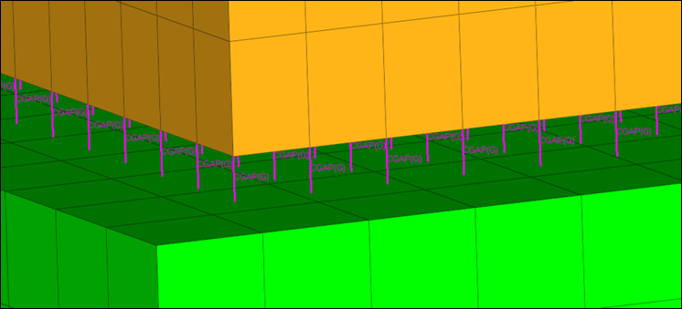
Figure 4.
- For small displacement analysis, N2S contact elements are created with CGAPG as the core.
- For Large displacement analysis, N2S contact elements consist of non-CGAPG cores.
- Each N2S contact element consists of a secondary node, a few main nodes, and one main face.
- Within a contact interface, secondary nodes should be unique to each N2S contact element. For instance, two different N2S contact elements cannot consist of the same secondary node.
- Within a contact interface, main faces can be shared among N2S contact elements.

Figure 5. Special Case - Main Surface Wraps Around a Secondary Node Set
Surface-to-Surface Discretization
The Surface-to-Surface Discretization approach involves the creation of contact elements linking the Main Surfaces to Secondary Surfaces.

Figure 6.
- One core secondary node
-

- Several secondary nodes surrounding the “core” secondary node

- One or more secondary faces including the secondary nodes and sharing the “core” secondary node
- Several main nodes
- One or more main faces including the main nodes
- One or more projections from the secondary faces to the main faces
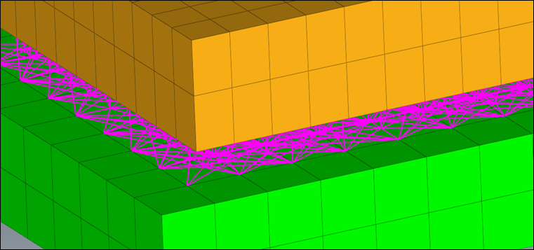
Figure 7.
- Multiple S2S contact elements have different “core” secondary nodes (that is, each S2S contact element has a unique “core” secondary node).
- Secondary face(s) may be shared among multiple S2S contact elements.
- Multiple S2S contact elements may share one or more main face(s).
- For N2S, it is recommended to use the finer mesh as the secondary.
- S2S is typically consumes higher computational time and memory resources compared to N2S; however, it typically can generate smoother contact pressure in many cases.
- If the secondary is a SET of GRID’s, then N2S should be used.
- N2S is recommended, if the secondary is a SET of solid elements. Alternately, the surfaces of solid elements can be used as the secondary for S2S.
- N2S is recommended if the secondary or main surface includes a corner. Alternately, the surfaces can be split into smaller smooth surfaces and used as main or secondary for S2S contact.
Node-to-Node Discretarization
The Node-to-Node Discretization approach involves the creation of contact elements linking the Main Surfaces to Secondary Surfaces.
The main surface should be defined using a GRID set. The N2N contact involves internally generated RBEAM JOINTG elements which connects main and secondary nodes together. The internally generated JOINTG elements can be output to the filename.n2n.fem file if CONTPRM,CONTOUT,YES is defined in the input file. This file can be imported to visualize the contact implementation.
Contact Implementation
Discretization of the contact interface into contact elements is the initial step towards incorporating the effect of contact in the solution process.
These contact elements are then automatically assigned attributes used to define the behavior of the contact interface, including the effect of the contact on the stiffness, boundary condition, and force matrices in the FEA solution. The following approaches are available:
Penalty-based Contact
The majority of contact implementation within OptiStruct involves the penalty-based process.
This can be activated using the CONTACT (PCONT, if necessary) and TIE Bulk Data Entries. The TIE entry supports both Penalty-based and Lagrange Multipliers-based formulations. Both Node-to-Surface (N2S) and Surface-to-Surface (S2S) discretization methods utilize this process to implement contact between parts. The discretized contact elements are assigned variable stiffness values (penalties) depending on the proximity of the contact surfaces to each other and the type of contact forces on the element. The primary purpose of the variable stiffness values is to minimize penetration of the contact surfaces.

Figure 8. Penalty-based Contact Element Force-Displacement Curves for Linear Analysis
Linear Penalty Curve (Nonlinear Analysis)
For Nonlinear Analysis, the contact status can change during the run, which implies that the contact element stiffness can switch between the closed (KA) and open (KB) values.

Figure 9. Penalty-based Contact Element Force-Displacement Curves for Nonlinear Analysis
| (1) | (2) | (3) | (4) | (5) | (6) | (7) | (8) | (9) | (10) |
|---|---|---|---|---|---|---|---|---|---|
| PCONT | PID | GPAD | STIFF | MU1 | MU2 | CLEARANCE | SEPARATION | ||
| FRICESL |
Nonlinear Penalty Curve (Nonlinear Analysis)
In the previous section, Linear Penalty Curve was discussed, wherein, the contact stiffness remains constant when either in the open or closed configuration, and only changes when the contact status is updated.
This may, in some small number of cases, lead to convergence difficulties due to the sudden and highly discontinuous nature of the stiffness change. To help smooth the stiffness change at the contact open/close location, nonlinear penalty curves can be used via the STFEXP and STFQDR continuation lines on the PCONT entry. Nonlinear penalty curves are currently applicable to N2S and S2S contact discretizations.
Exponential Nonlinear Penalty

Figure 10. Exponential Nonlinear Penalty Curve Has Three Regions
C0 and P0 are specified on the corresponding fields in the STFEXP continuation line. Kfinal and C1 are automatically determined by the C0, P0, and the STIFF fields.
Quadratic Nonlinear Penalty

Figure 11. Quadratic Nonlinear Penalty Curve Has Four Regions
- ALPHA1 = C1/ (Characteristic Length)
- ALPHA2 = (C2 + C0)/(C1 + C0)
- ALPA3 = Kinitial/Kfinal
The exponential and quadratic nonlinear penalty definitions are currently not applicable to FREEZE contact. They are also ignored for contacts in linear analysis.
Friction
In real-world applications, a majority of contact-based systems are affected by friction-induced shear stresses to varying degrees. Frictional effects occur when two surfaces come into contact and try to move tangentially relative to one another.
A variety of factors affect the amount of friction that exist between the surfaces. Friction is a function of the nature of the surfaces in contact (coefficient of static and kinetic friction) and the normal reaction at the contact interface (Normal force).
It is a highly nonlinear problem in finite element analysis, and should be utilized only if the inclusion of frictional effects is essential to the solution of the problem. The MUMPS solver is used in models involving friction. Friction effects generate unsymmetrical terms when surfaces slide relative to one another. These terms may have a strong influence in the overall displacement field. The unsymmetric solver (MUMPS) will be used by default when friction is specified. This may lead to slower convergence, however the results are accurate. The MUMPS solver can be turned off if frictional effects are not anticipated to be significant using PARAM,UNSYMSLV,NO.
Friction can be incorporated within the OptiStruct contact interface in two ways. The MU1 (and/or MU2) field on the PCONT Bulk Data Entry, or MU1 field on the CONTACT Bulk Data Entry. For Geometric Nonlinear Analysis (Radioss Integration), the FRIC field on the PCONTX/PCNTX# entries can be used. If these fields are not set, then the friction value on MU1 field on CONTACT/PCONT is used.

Figure 12.
Friction Models
- Model based on fixed slope KT
- Model based on Elastic Slip Distance (FRICESL, introduced in v12.0 and current default)

Figure 13. Comparison of the Two Friction Models for Contact Elements
- Model (a), based on fixed stiffness KT, is relatively simple, yet has certain drawbacks in modeling nonlinear friction. Namely, in Coulomb friction the frictional resistance depends upon normal force. Using fixed KT will predict different stick/slip boundaries for different normal forces, and thus may qualify the same configuration as stick or slip, depending on normal force.
- Model (b), based on Elastic Slip Distance, provides unique identification of stick or slip and generally performs better in solution of problems with friction. This model does require setting elastic slip distance FRICESL - for contact interfaces this value is calculated automatically by OptiStruct as 0.5% of typical element size on all Main contact surfaces.
The model (b), which is currently the default, is recommended for solution of nonlinear problems with friction. For backward compatibility, the model based on fixed KT can be activated by setting FRICESL=0 on PCONT or CONTPRM entries.
For Sliding Contact, the frictional force is always directed back to the point where the secondary and main first came into contact (changed status from open to closed). Its location is estimated using proportional interpolation between the current position and the last converged solution before penetration.

Figure 14. CONTACT Presumed Contact Surface

Figure 15. CONTACT Sliding with Friction

Figure 16. CONTACT Stick (zero sliding distance)
In practice, for contact interfaces that are initially open, AUTOSPC will effectively fix respective unsupported rotations. However, for contacts that are initially closed (for example, pre-penetrating contact with MORIENT=NORMAL) the frictional terms will prevent AUTOSPC from being effective. Therefore, respective SPC on rotations need to be applied manually to respective secondary nodes.
The above default setting can be changed using GAPPRM,GAPOFFS.
The presence of friction, due to its strongly nonlinear, non-conservative nature, may cause difficulties in nonlinear convergence, especially when sliding is present. If frictional resistance is essential to the solution of the problem and convergence problems are encountered, enforcing the stick condition (by setting KT > 0 and MU=0) may be a viable solution that will often result in better convergence than with Coulomb friction. Note however, that this only applies to problems in which minimal sliding is expected. In the case of larger sliding motions, the stick condition may lead to divergence through a "tumbling" mode.
Lagrange Multipliers (MPC-based)
MPC-based contact utilizes multi-point constraints (MPCs) to define a tied contact between the main and secondary surfaces.

Figure 17.
- Results of an MPC-based TIE contact analysis may not be accurate if there is a physical gap between the main and secondary surfaces. The 6 Rigid Body modes may not be proper in such cases.
- MPC-based TIE contact is currently not supported with MODCHG.
- MPC-based TIE contact is currently supported for Linear Static, Linear Transient, Nonlinear Static, and Nonlinear Transient Analyses. It is supported for both Small and Large Displacement Nonlinear Analyses.
Fast Contact (SUPORT-based and N2S Contact-based)
Fast Contact uses a different formulation when compared to the Penalty-based approach and the SUPORT-based contact.
This is applicable in cases where the only nonlinearities in the model arise due to Contact and the model includes small deformations and small sliding.
This is also not applicable to Large Displacement Nonlinear Analysis (LGDISP). There are two approaches to Fast Contact in OptiStruct.
SUPORT-based Fast Contact
If the only nonlinearity in the model is contact between parts and if the deformation at the contact interface resides within the small-displacement domain, SUPORT-based Fast Contact can be used to setup a linear solution using SUPORT and PARAM,CDITER.
Contact elements are not constructed, thereby avoiding the nonlinearities inherent in the penalty-based contact. The process involves applying constraints to grid points.
The penetration between the parts is avoided by limiting the relative displacement component in the normal contact direction at the contact interface to a positive value. Additionally, the force at the contact interface is also limited to a positive value, which avoids tension forces.
For SUPORT+MPC contact, the process initially assumes all contacts to be closed regardless of the position of the main and secondary. For SUPORT only contact, the initial contact status is all open. Then OptiStruct applies the constraints in an iterative process to avoid both penetration and tensile forces. An initial starting point depicting the contact status as 0.0 (open) or 1.0 (close) using DMIG, CDSHUT can also be provided (CDSHUT is supported only for SUPORT+MPC contact).
- Sliding friction is not allowed. Also, no nonlinear material and geometric nonlinearity are allowed.
- Inertia Relief cannot be used in conjunction with SUPORT-based Fast Contact.
- Subcase continuation with CNTNLSUB or Preloadiing/Buckling using FASTCONT option is not supported.
MPC Equation Setup
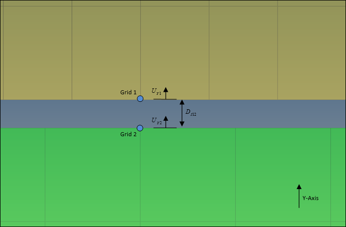
Figure 18.
MPC Equation
- Relative displacement between grid points 1 and 2 along the Y-Axis
- Initial contact gap between the grid points 1 and 2 along the Y-Axis
- Displacement of grid point 1 in the positive Y-Axis
- Displacement of grid point 2 in the positive Y-Axis
Since and are not inherently available in the model, SPOINT's are created to represent these quantities. is related to an SPC entry via SPOINT ID and the value of the initial contact gap is set on the D field on the SPC entry. is related to a SUPORT Bulk Data Entry via the SPOINT ID. PARAM,CDPCH can be used to control the printing of the final state of DMIG,CDSHUT after Fast Contact Analysis. PARAM,CDPRT can be used to control the printing of violations in intermediate iterations in Fast Contact Analysis.
Example: Input Deck
The following input deck illustrates the setup of a model with grid points 1 and 2 at an initial contact gap of 2.35.
$ Grid pointsGRID,1,,5.0,0.0,0.0
GRID,2,,0.0,0.0,0.0$ SPOINT for the contact gap monitoring
(D12)SPOINT,10 $ SPOINT for the initial contact gap value
(DI12)SPOINT,11$ SUPORT for the contact gap monitoring
(D12)SUPORT,10,0$ SPC to specify the initial contact gap value
(DI12)SPC,65,11,0,2.35$ MPC to realize the MPC equation that enforces the
constraintsMPC,75,1,2,-1.0,2,2,1.0
+,,10,0,1.0,11,0,-1.0$ PARAM, CDITER to activate the SUPORT-based Fast Contact
AnalysisPARAM,CDITERN2S Contact-based Fast Contact
N2S Contact-based Fast Contact is an alternative approach to Fast Contact when compared to the SUPORT-based Fast Contact.
The main advantage of this approach is that MPC equations, SUPORTs, SPCs are not required. Instead, the process of Contact Interface setup is exactly the same as in the case of the Nonlinear Static Analysis. The Contact Interface can be defined using the CONTACT Bulk Data Entry, with Node-to-Surface (N2S) discretization to generate the contact elements (Surface-to-Surface S2S discretization is not currently supported). OptiStruct then uses a new iterative approach to resolve the contact situation. The same limitations that apply to SUPORT-based Fast Contact also apply to N2S Contact-based Fast Contact. Additionally, only sliding contact without friction is currently supported. Also, no nonlinear material and geometric nonlinearity are allowed.
It is activated by simply adding PARAM,FASTCONT,YES in a model that contains a predefined contact interface.
Initial gap opening will be specified by U0 on PGAP and CLEARANCE on PCONT or CONTACT Bulk Data Entry.
Contact Interface Types
The next step after the contact interface is generated, contact elements are properly discretized, and the contact implementation type is selected as per the requirements of the problem, is the selection of the Contact Interface Type. This depends on the behavior being simulated at the contact interface.
Tie Interface
A Tie Interface enforces zero relative motion at the interface between two components or parts. The Tie Interface can be activated using the TIE entry (with CONTPRM,TIE,MPC). For more information, refer to the Lagrange Multipliers (MPC-based) section.
Freeze Contact
Freeze Contact enforces zero relative motion on the contact surface, the contact gap opening remains fixed at the original value and the sliding distance is forced to be zero. Additionally, rotations at the secondary node are matched to the rotations of the main patch. The FREEZE condition applies to all respective contact elements, regardless of whether they are open or closed. Freeze Contact can be activated using TYPE=FREEZE on the CONTACT, MU1=FREEZE on the PCONT entry or by using the Penalty-based Tied Contact. Penalty-based tied contact is activated by using the TIE entry for the contact interface (with CONTPRM,TIE,PENALTY, the default).
Sliding Contact
Sliding Contact has only normal contact stiffness at the contact interface and no frictional effects. It is only valid for small sliding without friction and applies to both open and closed contacts. If convergence difficulties arise, adding a small value of friction may help, or the STICK condition can be used. Sliding Contact can be activated using TYPE=SLIDE on the CONTACT entry.
Stick Contact
Stick contact is an enforced stick condition, wherein such contact interfaces will not enter the sliding phase. It only applies to contacts that are closed. In order to effectively enforce the stick condition, frictional offset may require to be turned off. Stick contact is activated using TYPE=STICK on the CONTACT entry or MU1=STICK on the PCONT entry. The contact stiffness value (KT) is equal to 0.1*STIFF in the case of Stick Contact.
Frictional Contact
For detailed information, refer to Friction.
Thermal Contact
For detailed information, refer to Thermal Contact Solver.
Fast Contact
For detailed information, refer to Fast Contact (SUPORT-based and N2S Contact-based).
Contact Interface Parameters (Contact Control)
Orientation of Contact Pushout Force (MORIENT)
The orientation of the contact pushout force from the main surface can be defined on the MORIENT field on the CONTACT entry. It applies only to main that consist of shell elements or patches of grids. Main defined on solid elements always push outwards irrespective of this flag. MORIENT is the direction of contact force that main surface exerts on secondary nodes.
It is important to note that, in most practical applications, leaving this field blank will provide correct resolution of contact, irrespective of the orientation of surface normals. Only in cases of main surfaces defined as shells or patches of grids, and combined with initial pre-penetration, is MORIENT needed.
- In OPENGAP (default when TRACK is not
set to FINITE/CONSLI), the pushout
direction is defined using the assumption that the gap between secondary and
main is initially open, and the contact condition should prevent their
contact (gap padding GPAD from the
PCONT card is ignored in defining the pushout
direction - this direction is based strictly on the positions of main and
secondary nodes).

Figure 19. OPENGAP Example - OVERLAP assumes the reverse, namely that the secondary
and main bodies are already overlapping and the contact condition should
push them apart (this is useful in pre-penetrating models when the entire
secondary set is pre-penetrating into the main object).

Figure 20. OVERLAP Example - With the NORM option (default for
TRACK=FINITE/CONSLI),
the pushout force is oriented along the normal vector to the main surface.
(The surface normal may be reversed relative to the default normal to a
shell element, if a FLIP flag is present on the main SURF
definition. This behavior corresponds to that of the reverse
normals checkbox on the contactsurfs
panel in HyperMesh). In cases when the secondary
node does not have a direct normal projection onto the main surface, and the
"shortest distance" projection is used (GAPGPRJ set to
SHORT on the GAPPRM card), the
pushout force is oriented along the shortest distance line, yet with the
orientation aligned with the normal vector.

Figure 21. NORM Example - REVNORM creates pushout force reversed relative to the NORM option.
By default, MORIENT does not apply to mains that are defined on solid elements - such mains always push outwards. This can be changed by choosing CONTPRM,CORIENT,ONALL which extends the meaning of MORIENT to all contact surfaces. In which case, it should be noted that the default normal is pointing inwards unless a FLIP flag appears on the main SURF definition for surfaces on solid elements, making the surface normal point outwards. (When creating contact surfaces in HyperMesh, this behavior corresponds to that of the reverse normals checkbox on the contactsurfs panel).
Search Distance (SRCHDIS)
The SRCHDIS field on the CONTACT and TIE entries is the search distance criterion for creating the contact interface. When specified, only secondary nodes that are within the SRCHDIS distance from the main surface will have the contact condition checked.
The default value is equal to twice the average edge length of the main surface. For FREEZE contact, it is equal to half the average edge length.
For shell elements, the contact and tie search considers the shell thicknesses. Which implies that the defined search distance is expected to be the true distance between the shell surfaces facing each other. For example, in the case of shells without offset, if the geometric distance between the two shell surfaces facing each other is 5.0, and the shell thicknesses are 2.0 each, then the actual distance between the shell surfaces facing each other is 3.0. If the Search distance field is now set to 3.0, then the contact is generated as expected (in this scenario, if SRCHDIS is set lower than 3.0, then there is no contact generated).
Contact Adjustment (ADJUST)
- NO
- No adjustment (default).
- AUTO
- A real value equal to 5% of the average edge length on the main surface is internally assigned as the depth criterion.
- Real > 0.0
- Value of the depth criterion which defines the zone in which a search is conducted for secondary nodes (for which contact elements have been created). These secondary nodes (with created contact elements) are then adjusted onto the main surface. The assigned depth criterion is used to define the searching zone in the pushout direction.
- Integer > 0
- Identification number of a SET entry with TYPE=GRID. Only the nodes on the secondary entity which also belong to this SET will be selected for adjustment.
The adjustment of secondary nodes does not create any strain in the model. If DISCRET=N2S is selected, it is treated as a change in the initial model geometry. If DISCRET=S2S is selected, it is treated as a change in the initial contact opening/penetration.
If a node on the secondary entity lies outside the projection zone of the main surface, it will always be skipped during adjustment since no contact element has been constructed for it.
Contact interface padding, GPAD (on the PCONT entry) is used to determine the direction and distance of secondary node adjustment. GPAD is also used to augment the searching zone for adjustment. If the MORIENT field is OPENGAP or OVERLAP while the GPAD field in the referred PCONT entry is NONE or zero, the nodal adjustment will be skipped, since for OPENGAP or OVERLAP there is no way to decide the main pushout direction if secondary nodes are adjusted to be exactly on the main face.
- The ADJUST field must be set to NO for self-contact.
- If a real value (the searching depth criterion for adjustment) is input for
the ADJUST field, a searching zone for adjustment is
defined. If GPAD is also defined, then the value of
GPAD augments the searching zone for
ADJUST (see Figure with GPAD
below). The secondary nodes in this searching zone, for which contact
elements have been created, will be adjusted. If ADJUST
is larger than or equal to SRCHDIS, all the secondary
nodes for which contact elements have been created, will be adjusted.

Figure 22. No Contact Interface Padding (GPAD)
Figure 23. With Contact Interface Padding (GPAD)Note: The depth criterion (A non-negative real value for ADJUST) is used to define the searching zone for adjustment, as shown above. If GPAD is defined, then the value of GPAD is also used to augment the searching zone for ADJUST, as shown in the image above. This searching zone is created in the pushout direction up to a distance equal to the value of the ADJUST field. The secondary nodes within the searching zone (with defined contact elements) are then considered for adjustment based on the rules specified within this section. - If the ADJUST field is set to an integer value (the identification number of a grid SET entry), the nodes shared by the secondary entity and the grid SET will be checked for contact creation, that is, SRCHDIS will be ignored for these nodes, and then adjusted if a projection is found. The nodes belonging to the grid SET but not to the secondary entity will be simply ignored.
Contact Clearance (CLEARANCE)
Clearance can be defined on the CONTACT or PCONT entries on the CLEARANCE field. It can also be defined via U0 on the PGAP entry. Clearance does not physically move the nodes. The contact is considered to be closed, if the clearance between the two surfaces is equal to (or less than) the specified clearance, regardless of the physical location of the nodes. Make sure that the surface nodes are not highly irregular or the actual physical distance between some (or all) parts of the surfaces is much greater than the specified clearance. The resulting contact parameters applied to the actual physical nodes after each iteration or over the entire solution may be inaccurate in such cases. A blank clearance field is the same as U0=AUTO.
Using CLEARANCE overrides the default contact behavior of calculating initial gap opening from the actual distance between Secondary and Main. CLEARANCE is now equal to the distance that Secondary and Main have to move towards each other in order to close the contact. Negative value of CLEARANCE indicates that the bodies have initial pre-penetration.
- CLEARANCE on the CONTACT entry cannot be used in conjunction with PID of the PCONT entry. In this case, clearance must be specified on the PCONT entry.
- The consideration of SRCHDIS in presence of CLEARANCE can be controlled using the SRCHDCLR entry in system settings (SYSSETTING) or in the Solver Configuration File (.cfg) file.
Contact Smoothing (SMOOTH)
- If SMSIDE is MAIN and SMREG is ALL (or same as MSID), there must be only one SMOOTH continuation line to define smoothing of the Main side.
- If SMSIDE is SECOND and SMREG is ALL (or same as SSID), there must be only one SMOOTH continuation line to define smoothing of the Secondary side.
- If SMSIDE is BOTH, SMREG must be ALL and there must be only one SMOOTH continuation line.
- Smoothing is now supported for both N2S and S2S contact.
Finite Sliding (TRACK)
Finite Sliding (TRACK=FINITE or CONSLI) option is currently supported only if TYPE=SLIDE or if friction (via MU1/CONTPRM/PCONT) is defined.
For TRACK=FINITE, the contact search is conducted for every load increment, while with TRACK=CONSLI, termed continuous sliding, the search is done for every iteration. The CONSLI option is expected to produce more accurate results and, in some cases, better convergence robustness, especially when very large sliding and/or distortion is present.
For non-solid elements, the MORIENT field should not be set to OPENGAP or OVERLAP for Finite Sliding (FINITE/CONSLI). If CONTPRM,CORIENT,ONALL is active, MORIENT is applied to solid elements. In such cases, MORIENT should not be set to OPENGAP or OVERLAP for solid elements also.
- Finite Sliding (FINITE/CONSLI) is effective only for Large Displacement Nonlinear Analysis.
- Finite Sliding (FINITE/CONSLI) works only with Hash Assembly and the MUMPS solver. Hash Assembly (PARAM,HASHASSM,YES) is automatically turned on for Large Displacement Nonlinear Analysis.
- Finite Sliding (only CONSLI) is supported for Self-Contact.
Contact Interface Padding (GPAD)
"Padding" of the interface to account for additional layers, such as shell thickness. This value is subtracted from the contact gap opening as calculated from the location of nodes. It is set on the GPAD field of the CONTACT and PCONT entries. CLEARANCE cannot be set in conjunction with (non-zero) GPAD. Blank GPAD field in presence of CLEARANCE is interpreted as NONE.
The initial contact gap opening is calculated automatically based on the relative location of secondary and main nodes (in the original, undeformed mesh). To account for additional material layers covering main and secondary objects, the GPAD entry can be used. GPAD option THICK automatically accounts for shell thickness on both sides of the contact interface (this also includes the effects of shell element offset ZOFFS or composite offset Z0), when the main and/or secondary are shell surfaces (SET of shell element types or SURF of shell element faces). The THICK option will only apply automatic padding if shells are selected for main/secondary in the contact interface (for example, padding is not applied for "skinned" solid elements that are selected as a main/secondary in the contact interface).
Contact Stabilization (CNTSTB entry and PARAM,EXPERTNL,CNTSTB)
Defines parameters for stabilization control of surface-to-surface contact and large displacement node-to-surface contact. A CNTSTB Bulk Data Entry should be referenced by a CNTSTB Subcase Information Entry to be applied in a particular Subcase. Also, PARAM,EXPERTNL,CNTSTB can be used to apply contact stabilization.
Resolution of Pre-penetration (CONTPRM,SFPRPEN)

Figure 24.
In the case above, the Secondary node will be identified as if pre-penetrating the Main face, while in reality it is on the other side of the same solid body. The result from nonlinear CONTACT solution will be such that this portion of the body will be "squeezed" to have practically zero thickness, with very high stresses obviously resulting.
Apart from correctly identifying potential Secondary and Main sets, a possible remedy to avoid such situations is to make sure that SRCHDIS is smaller than minimum thickness of the solid bodies which are enveloped by self-contacting surfaces.
Contact Friendly Elements (CONTFEL)
Contact friendly elements can be activated using PARAM,CONTFEL,YES. Contact-friendly TETRA10, HEXA20, and PENTA15 elements are available and can be combined in a single model. Modified shape functions are used for possible improved runs with contact friendly elements.
No Separation Contact (SEPARATION)
Flag indicating whether the main and the secondary can separate once the contact has been closed. This is set on the PCONT Bulk Data Entry, via the SEPARATION field. If SEPARATION is set to NO, then the main and secondary do not separate after contact is closed. Applied only to frictional, SLIDE and STICK contacts with S2S or large-displacement N2S.
Self-Contact
- Main and secondary Set Identification numbers can point to the same set.
- Main Set Identification number can be blank.
- Surfaces which after large deformation can come into contact with themselves (for example, large buckling deformations). In such situations, some material can collapse onto itself, and it is usually difficult to decide which part will be in contact.
- When a lot of potential contact pairs (main-secondary) can exist and it is not feasible to define all of them manually.
- Self-Contact can be tried, if manual contact setup fails for some reason.
- Models can have multiple areas of Self-Contact.
- Same model can have regular contact/TIE in other areas of the model.
- Currently only Continuous Sliding (CONSLI) is supported. Both N2S and S2S contact are available with Self-Contact.
Special Contact Applications
Based on the various contact properties and implementations, the following special or dedicated Contact Applications are available in OptiStruct.
Pretensioned Bolt Analysis
If the main facet of a contact projection includes a grid on any pretension cutting surface, this contact projection will be included for consideration of contact. For additional detailed information, refer to Pretensioned Bolt Analysis in the User Guide.
Threaded Bolt
Threaded bolts can be defined as part of a CONTACT interface by setting the CLEARANCE field to reference a CLRNC Bulk Data Entry. For additional detailed information, refer to the CONTACT and CLRNC Bulk Data Entries.
Contact Interference
Contact interference controls how initial contact penetration is resolved. Contact interference is turned on automatically for a subcase with contact. The way such initial contact penetration is resolved is handled using the CNTITF Subcase and CNTITF Bulk Data Entries.
Optimization with Contact
All Optimization types and all responses (wherever applicable) are available for optimization when contact is present. Topology, Topography, Size, Shape, Free-Shape, and Free-Size optimization types are all supported. Freeze contact with large shape changes is available for optimization.
- Negative compliance may occur for some contacts due to initial penetration which may produce negative contributions to the global compliance.
- Optimization is not possible with negative compliance (contact is releasing energy instead of storing it).
- To turn OFF contributions of CONTACT/GAP elements to the compliance calculation, use GAPPRM,GAPCMPL,NO.
- Contacts with negative clearance can be redefined to resolve initial penetrations.
- Contact interfaces can be modified with ADJUST to smooth out the penetrations.
Contact with Preload
Preloading effects can be considered in Nonlinear Contact Analysis. Initial stress and load stiffness effects due to preload from nonlinear static subcases will be accounted for with STATSUB(PRELOAD) in frequency extraction or linear static subcases. A pretension subcase can also be considered for preload. Only S2S contacts are supported for such cases. CNTNLSUB is not required for the preloading subcase. For further detailed information, refer to Prestressed Linear Analysis in the User Guide.
Output from Contact Analysis
The CONTF I/O Options and Subcase Information Entry can be used to request contact results output for all nonlinear analysis subcases or individual nonlinear analysis subcases, respectively.
The NLOUT entry can be used to request incremental output from a Nonlinear Analysis. Additionally, if an NLOUT entry is specified in the model (and referenced in a subcase), then OptiStruct outputs, by default, for large displacement nonlinear analysis, the history of strain energy and contact stabilization energy to data files which can be plotted with HyperGraph. The HyperGraph main file is entitled filename_nlm.mvw and the HyperGraph data files (in ASCII format) are entitled filename_e.nlm.
See Also:
OS-T: 1360 NLSTAT Analysis of Gasket Materials in Contact
OS-T: 1365 NLSTAT Analysis of Solid Blocks in Contact
OS-T: 1390 Pretensioned Bolt Analysis of an IC Engine Cylinder Head, Gasket and Engine Block System
OS-T: 1392 Node-to-Surface versus Surface-to-Surface Contact