HS-1030: Parameterize a MotionView Model
Learn how to use HyperStudy to perform an optimization with MotionSolve.
Before you begin, copy the model files used in
this tutorial from <hst.zip>/HS-1030/ to your working
directory.
- Input Variable
- The input variable is the angle q (swing angle) of the pendulum.
- Output Response
- The output response target is to achieve Y-velocity of 6m/s at the tip of the pendulum.
- Objective
- At the end of this tutorial, you will know how to:
- Use MotionView to start HyperStudy and create the input variables.
- Set up a study.
- Run a system identification optimization study.
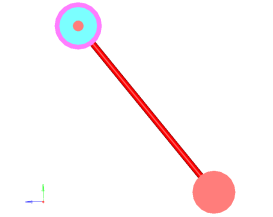
Figure 1.
Perform the Study Setup
-
Start a new study in the following ways:
- From the menu bar, click .
- On the ribbon, click
 .
.
-
Add a MotionView model.
-
From the Directory, drag-and-drop the MotionView (.mdl) file
Pendulum.mdl into the work area.
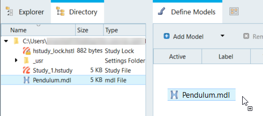
Figure 2.
-
From the Directory, drag-and-drop the MotionView (.mdl) file
Pendulum.mdl into the work area.
-
In the Model Parameters dialog in MotionView, select parameters to import into HyperStudy.
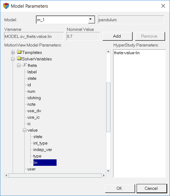
Figure 3. -
In the work area, modify the input variable's bounds.
- Change the Lower Bound to 0.
- Change the Upper Bound to 2.

Figure 4.
Perform Nominal Run
Create and Evaluate Output Responses
In this step you will create one output response.
-
Define the following options, and then click Next.
- Set Type to Marker Velocity.
- Set Request to REQ/70000002 Pendulum body from Ground Body(tip velocity).
- Set Component to VY.
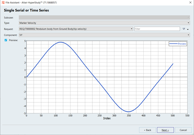
Figure 5. -
Click Finish.
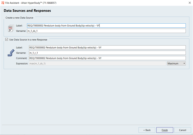
Figure 6.The output response is displayed in the work area.
Run System Identification Optimization
-
Assign an objective to the output response.
- Go to the step.
- Click the Objectives/Constraints - Goals tab.
- Click Add Goal.
- In column Type, select More.
- In column 1, select System Identification.
- In column 2, change the target to 6.0.

Figure 7. -
View the iteration history of the Optimization in the following ways:
Use the Channel selector to select input variables, output responses, goals, and so on to display.
- Click the Iteration History tab to view a table
with the Optimization's iteration results.Note: The optimal design is highlighted in green.
- Click the Evaluation Plot tab to compare all of the entities of the Optimization (input variables, output responses, and objectives) against the iteration.
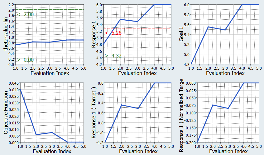
Figure 8. Evaluation Plot - Click the Iteration History tab to view a table
with the Optimization's iteration results.
-
Post-process the Optimization.
The Post-Processing step in an optimization approach offers additional tools to review the results. Statistics, histograms, and scatter plots can be used to help compare and analyze designs.
-
Click the Integrity tab to view a series of
statistical measures on input variables and output responses.
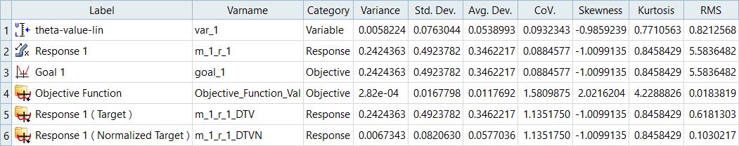
Figure 9.
-
Click the Integrity tab to view a series of
statistical measures on input variables and output responses.