HS-1035: Optimization Study using an Excel Spreadsheet
Learn how to use couple HyperStudy with a spreadsheet, identify input variables and output responses, and run an Optimization study.
- Problem formulation
-
- Find the cross-sectional dimension's width and height in mm.
- Minimize the beam volume such that the tip deflection < 0.53 mm.
Review the Excel Spreadsheet
When you create an Excel spreadsheet model, it is important that the spreadsheet is formatted correctly. A variable's value and label can be formatted in two consecutive rows or two consecutive columns. Variable labels should only contain English characters, or a combination of English characters and numbers. If a label is not created for a variable, HyperStudy will assign one by default.
- In Excel, open the hst_tut_1035(1070)_spreadsheet.xls file.
- Review the information, and locate the columns that contain the input variables and output responses.
Perform the Study Setup
-
Start a new study in the following ways:
- From the menu bar, click .
- On the ribbon, click
 .
.
-
Add a Spreadsheet model by dragging-and-dropping the
hst_spreadsheet_integration_example file from the
Directory into the work area.
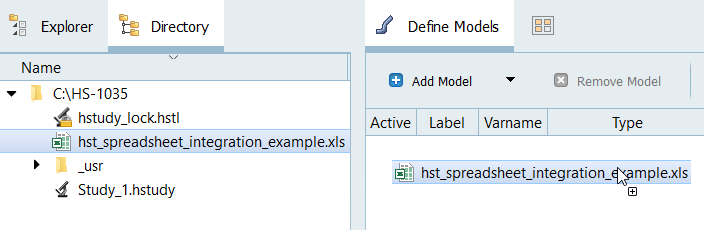
Figure 1.The Resource and Solver input file fields become populated. The Solver input file field displays hst_input.hstp, this is the name of the solver input file HyperStudy writes during an evaluation. -
Add input variables.
-
In the Excel dialog, click
Yes to begin selecting input variables.
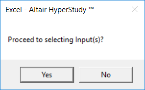
Figure 2. -
In the spreadsheet, select the cells that contain the input variable's
labels and values.
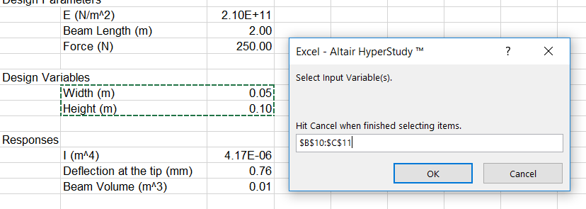
Figure 3.
-
In the Excel dialog, click
Yes to begin selecting input variables.
-
Add output responses.
-
In the spreadsheet, select the cells that contain the output response's
labels and values.
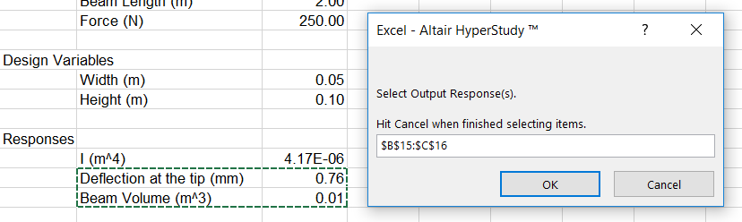
Figure 4.
Two input variables and two output responses are imported from the hst_tut_1035(1070)_spreadsheet.xls spreadsheet. -
In the spreadsheet, select the cells that contain the output response's
labels and values.
Perform Nominal Run
Review Output Responses
-
Review the output responses imported into the study.
The output responses were extracted from the hst_output.hstp file, which HyperStudy created for each run.
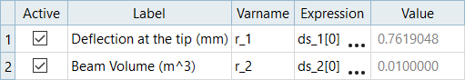
Figure 5.
Run Optimization
-
Apply a set range of +17% to both input variable's lower and upper
bounds.
-
In the Lower Bound column of both input variables, click
 .
.
- In the Percent field, enter +17.
- Click the +/- button.
- Click Apply.
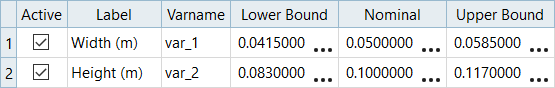
Figure 6. -
In the Lower Bound column of both input variables, click
-
Assign an objective to the Beam Volume (m^3) output response.
- Click Add Goal.
- In the Apply On column, select Beam Volume (m^3).
- In the Type column, select Minimize.

Figure 7. -
Assign a constraint to the Deflection at the tip (mm) output response.
- Click Add Goal.
- In the Apply On column, select Deflection at the tip (mm).
- In the Type column, select Constraint.
- In column 1, select <= (less than or equal to).
- In column 2, enter 0.53.
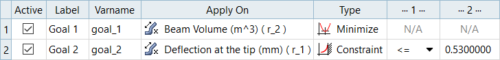
Figure 8. -
Review the values of input variables, output responses, objective functions,
and constraints for all runs evaluated during the optimization.
- Click the Evaluation Data tab to view a detailed summary of all input variable and output response run data in a tabular format.
- Click the Evaluation Plot tab to plot a 2D chart of the input variable and output response values for each run.
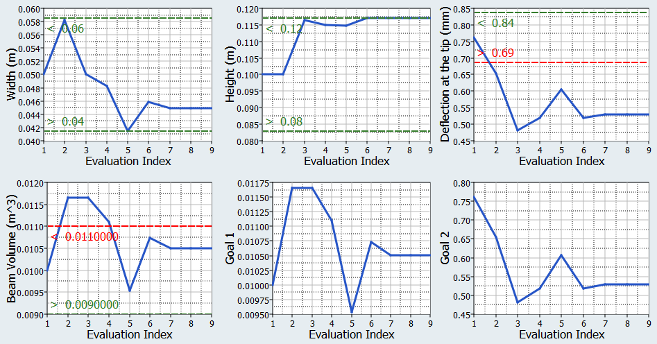
Figure 9. Evaluation Plot -
Review the values of the input variables, output responses, objective function,
and constraints for each iteration during the Optimization.
Use the Channel selector to select input variables, output responses, goals, and so on to display.
- Click the Iteration History tab to view a
detailed iteration history summary.As this study was run with ARSM, you will see the same designs in both the Evaluation Data and Iteration History. From the iteration table, you can see that iterations 1, 2, and 5 are displayed in a red font, which indicates that these iterations have a constraint violation. The constraint that is violated, Constraint 1, is displayed in a red, bold font. Iterations 3, 4, and 6-8 are feasible, but not optimal designs. The ninth iteration, highlighted in green, indicates that this design is the optimal design.
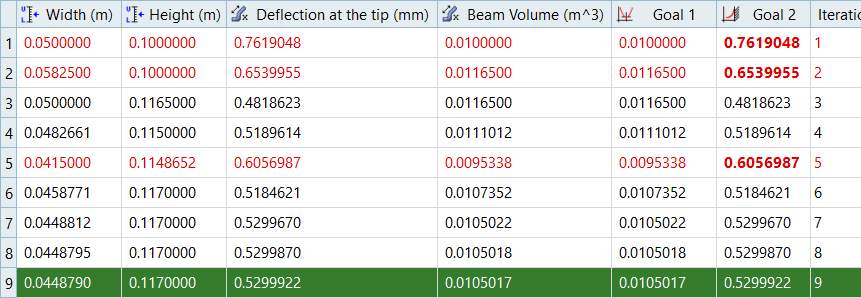
Figure 10. - Click the Iteration Plot tab to plot the
iteration history.
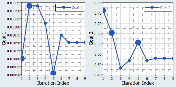
Figure 11. Iteration Plot for Goal 1 (Objective) and Goal 2 (Constraint). In the first plot (Goal 1), infeasible designs are identified with bigger markers. In the second plot (Goal 2), you can see these designs have higher displacement values than the constraint bound of 0.53 and only the last three designs meet the constraint bound.
- Click the Iteration History tab to view a
detailed iteration history summary.