Panel 2 : Dynamic identification
Overview of the Dynamic identification panel
MILS's second panel is depicted in Figure 1. It provides the user with ten actions or steps to complete a dynamic LS identification, as indicated by labels 2.1 to 2.10 in that figure. The mandatory steps are labeled in blue, while the optional actions are displayed in yellow.
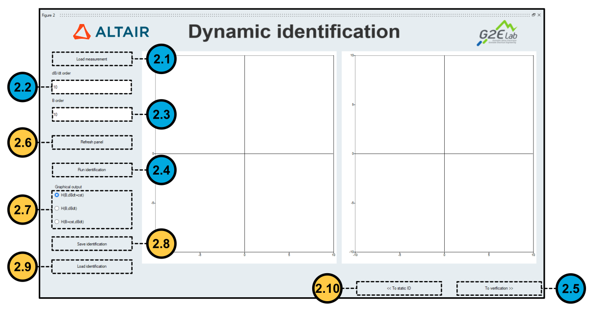 Figure 1. MILS's dynamic identification panel.
Mandatory steps in dynamic identification
A dynamic identification consists of a five-step procedure in MILS. The mandatory steps are described below:
- Step 2.1: Click on button Load measurement, which is labeled as
2.1 in Figure 1. MILS opens
a dialog box asking for measurement files. The user must here provide a set of
measurement files representing a certain number of dynamic hysteresis loops of
the steel sheet.Note: The files used in the dynamic identification step share the same format of the files used in Step 1.2 of the static identification. However, they are supposed to represent hysteresis loops measured under different experimental circumstances (i.e., higher frequencies and peak magnetic flux density reaching saturation). A detailed description of MILS's input formats and a discussion on the differences between the static and dynamic file sets are available here.Note: If the measurement files are loaded correctly, MILS will display the measurements provided by the user in the Curves preview window, as shown in Figure 2.
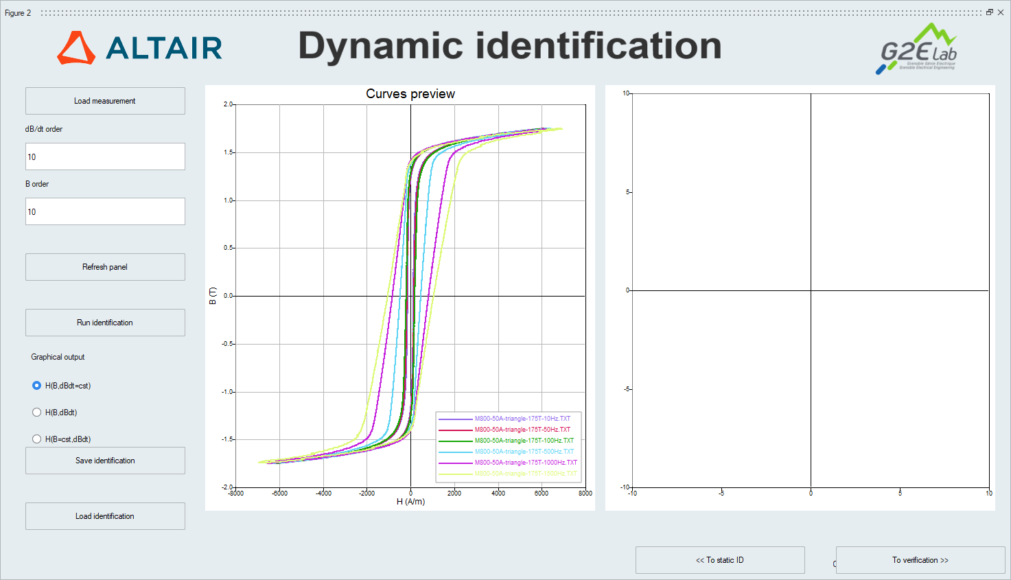 Figure 2. Hysteresis loop measurements displayed at the Curve
preview window of the Dynamic Identification panel in
MILS.
Figure 2. Hysteresis loop measurements displayed at the Curve
preview window of the Dynamic Identification panel in
MILS. - Step 2.2: Provide an integer number in the field dB/dt order, which is labeled as 2.2 in Figure 1. This number represents the order of the polynomial interpolation employed by MILS to represent the time derivative of function B(t), which describes the variation of the magnetic flux density in a dynamic identification.
- Step 2.3: Analogously, enter an integer number in the field B
order (labeled as 2.3 in Figure 1). This number represents the order of the polynomial
interpolation employed by MILS to represent the magnetic flux density as a
function of time in a dynamic identification.Note: The order of the polynomials representing B(t) and dB/dt provided in steps 2.2 and 2.3 must be between 4 and 20.
- Step 2.4: Launch the dynamic identification by clicking on the Run
identification button, which is labeled as 2.4 inFigure 1.Note: A pop-up window appears at the end of the computation to announce the end of the dynamic identification procedure, as shown in Figure 3.
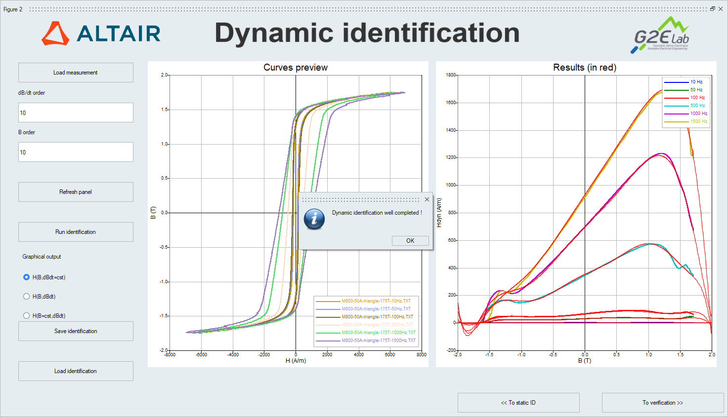 Figure 3. A pop-up message announces the end of a successful dynamic
identification.Note: The results are displayed automatically in the Results window, as shown in Figure 3. The curves in red represent the reconstruction provided by the identified dynamic model, while the colored curves correspond to the measurement files .Note: The user may consider adjusting the orders of the polynomial interpolations of steps 2.3 and 2.3 iteratively by observing the reconstructed curves in the Results window.
Figure 3. A pop-up message announces the end of a successful dynamic
identification.Note: The results are displayed automatically in the Results window, as shown in Figure 3. The curves in red represent the reconstruction provided by the identified dynamic model, while the colored curves correspond to the measurement files .Note: The user may consider adjusting the orders of the polynomial interpolations of steps 2.3 and 2.3 iteratively by observing the reconstructed curves in the Results window. - Step 2.5: Once the dynamic identification is completed, click on button To verification (labeled as 2.5 in Figure 1) to continue to the Overall Verification panel of MILS and proceed with the LS model identification.
Optional actions in dynamic identification
- Refresh Panel: Clicking on button Refresh Panel (labeled as 2.6 in Figure 1) refreshes the Curve preview and Results windows. Use this action to reset zoom settings and to change the colors of the displayed data sets in those windows.
- Change graphical output: After completing step 2.4 (Run
identification), the user may change the format of the graphical output
displayed in the Results windows. The three options available (labeled as
2.7 in Figure 1) are:
- H(B,dB/dt = cst): displays the behavior of the dynamic component of the reconstructed magnetic intensity H as a set of curves. Each curve is given by a single-variable function of magnetic flux density B for different constant values of time derivative dB/dt.
- H(B,dB/dt): displays the behavior of dynamic component of the reconstructed magnetic intensity H as a surface. This surface is given by a two-variable function relating H to magnetic flux density B and its time derivative dB/dt.
- H(B=cst,dB/dt): displays the behavior of the dynamic component of the reconstructed magnetic intensity H as a set of curves. Each curve is given by a single-variable function of time derivative dB/dt, for different constant values o magnetic flux density B.
- Save or Load Identification:After completing steps 2.1 to 2.4, the user may save the static identification results for a later user by clicking on button Save Identification, marked as 2.8 in Figure 1. The saved results are stored in a MAT file (i.e., in Compose's workspace format). Conversely, a MAT file containing static identification results may be loaded by clicking on button Load Identification (labeled as 2.9 in Figure 1).
- Return to static identification: The user may return to the Static Identification step by clicking on button To static ID. This button is marked as 2.9 in Figure 1.
Further reading
LS model identification with MILS
How to use MILS to generate an LS model
Panel 1: Static identification
Panel 4: Model generation for Flux
MILS's input and output files formats