Panel 4 : Model generation for Flux
Overview of the Model generation panel
A picture displaying the fourth panel of MILS is available in Figure 1. This panel provides the user with an interface to export the identified LS model in a format compatible with Altair Flux. The user may also use this panel to generate an iron loss map of the steel sheet, that is, a table containing estimations of the iron loss density developed in the bulk of the steel sheet (in W/kg).
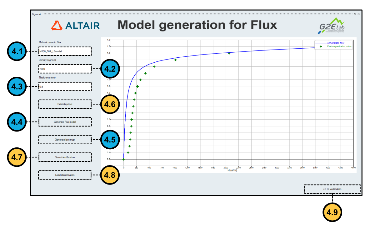 Figure 1. MILS's Model generation for Flux panel.
Exporting the LS model to Flux
Exporting the model to Flux also generates a report of the identification automatically. While the LS model is exported to a .mils file, the report is saved in a text file.To generate these files, the user must execute the steps below:
- Step 4.1: Type a name for the sheet subjected to LS identification in the
field Material name in Flux (labeled as 4.1 in Figure 1).
Note: This name becomes the material identifier in Flux associated with the steel sheet. It must contain only letters and numbers. The underscore character "_" is also allowed.
- Step 4.2: Provide the density (kg/m3) of the steel sheet in the field Density (labeled as 4.2 in Figure 1).
- Step 4.3: Enter the thickness of the steel sheet (mm) in the field Thickness (marked as 4.3 in Figure 1).
- Step 4.4: Click on button Generate Flux Model. A dialog box asking
for a file name and a path appears. This file can be loaded as a Flux material
as explain in this page : Isotropic soft material : Iron sheets described by LS modelNote: Two files are generated by completing the actions required by this dialog box. While the .mils file containing the identified model receives the name provided by the user in the dialog box, the .txt file containing the report will receive the same name, followed by the string identification_report.
Exporting the iron losses map of the steel sheet.
The iron loss map of a steel sheet is a table of iron loss density values (W/kg) given as a function of the frequency (Hz) and of the peak magnetic flux density (T).
To create this map, MILS uses the identified LS model to reconstruct hysteresis loops admitting sinusoidal time variations of the magnetic flux density. The frequency and the peak magnetic flux density ranges are fixed and cover values relevant to the design of electromechanical devices (from 0.1 T to 1.8 T and from 50 Hz to 1000 Hz, respectively).
To export the iron losses map of a steel sheet after performing a full LS identification:
- Click on button Generate loss map, which is labeled as 4.5 in Figure 1.
- In the dialog box, choose a name and a path to save the Excel file containing the iron loss map.
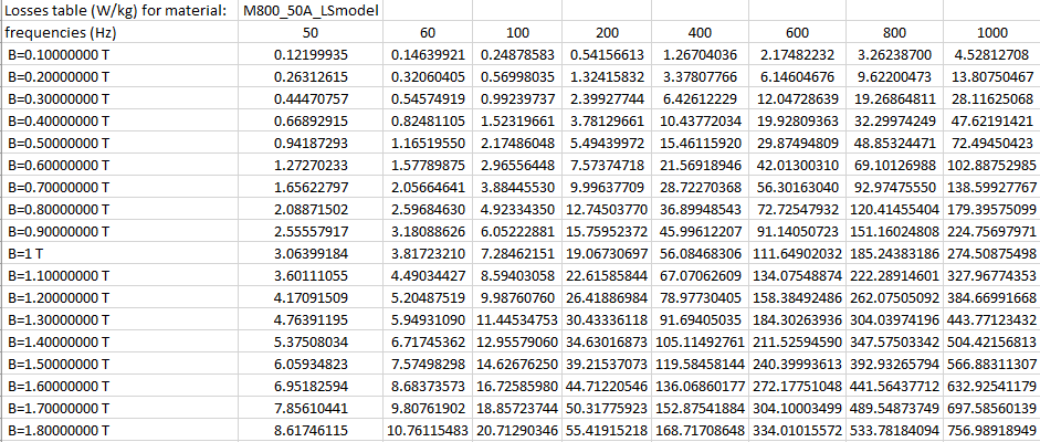 Figure 2. Example of an iron loss map in Excel format exported by MILS.
Additional actions available in the Model generation panel
- Refresh Panel: Clicking on button Refresh Panel (labeled as 4.6 in Figure 1) refreshes the plots of the first magnetization curve and the anhysteretic curve displayed in the panel. Use this action to reset zoom settings.
- Save or Load Identification: The user may save his current progress for later use by clicking on button Save Identification, marked as 4.7 in Figure 1. The saved results are stored in a MAT file (i.e., in Compose's workspace format). Conversely, he may load his saved work by clicking on button Load Identification (labeled as 4.8 in Figure 1).
- Return to Overall identification: The user may return to the Overall verification step by clicking on button To verification. This button is marked as 4.9 in Figure 1.
Further reading
LS model identification with MILS
How to use MILS to generate an LS model
Panel 1: Static identification
Panel 2: Dynamic Identification
MILS's input and output files formats