Panel 3 : Overall verification
Overview of the Overall verification panel
MILS's third panel is shown in Figure 1. In this panel, the user may perform an optional overall verification of the identified LS model. This overall verification consists of reconstructing a measured hysteresis loop by using the full LS model yielded by the previous identification steps. MILS then compares the inner surfaces of the measured and reconstructed hysteresis loops (i.e., their associated iron losses) to estimate the quality of the identified LS model.
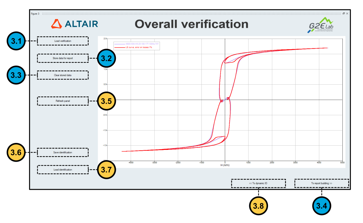 Figure 1. MILS's Overall verification panel.
How to perform an Overall verification of the identified LS model
- Step 3.1: Click on button Load verification (labeled as 3.1 in
Figure 1) to
load a file containing the measurements representing the hysteresis loop to be
reconstructed. Note: The hysteresis loop reconstructed at this step needs only to be periodic, and is not constrained by any other frequency or peak magnetic flux density requirements. The imposed B(t) signal during data acquisition may even include harmonics of the fundamental frequency.Note: The format of the measurement file provided in this step is the same used in the two previous identification steps. In the case of complex hysteresis loops, the user must make sure that the frequency parameter in the loaded measurement file corresponds to the fundamental frequency.Note: Differently from the previous identification steps, only one measurement file should be loaded at a time for reconstruction.Note: Once the measurement file is loaded, the reconstructed loop is evaluated and displayed together with the measured loop (plotted in red) in the panel, as shown in Figure 1. An error value is also displayed in the legend of the plot; it estimates the difference between the iron losses evaluated with the original and reconstructed loops (i.e., the inner surfaces of the loops).
- Step 3.2: After completing step 3.1, the user may ask MILS to store the overall verification results (i.e., the evaluated iron losses error and the name of the input measurement file). This data will be saved in the report generated in the last step of the identification(MILS's fourth panel: Model generation for Flux). To do so, click on button Store data for report (labeled as 3.1 in Figure 1).
- Step 3.3: If needed, click on button Clear stored data (marked as 3.3 in Figure 1) to clear the data that would be exported in the report mentioned in step 3.2.
- Step 3.4: Proceed to the final step of the LS identification by clicking on button To report building, which is marked as 3.4 in Figure 1.
Additional actions available in the Overall verification panel
- Refresh Panel: Clicking on button Refresh Panel (labeled as 3.5 in Figure 1) refreshes the plotted data in the panel. Use this action to reset zoom settings and to change the colors of the displayed data sets in those windows.
- Save or Load Identification: The user may save his current progress for later use by clicking on button Save Identification, marked as 3.6 in Figure 1. The saved results are stored in a MAT file (i.e., in Compose's workspace format). Conversely, he may load his saved work by clicking on button Load Identification (labeled as 3.7 in Figure 1).
- Return to dynamic identification: The user may return to the Dynamic identification step by clicking on button To dynamic ID. This button is marked as 3.8 in Figure 1.
Further reading
LS model identification with MILS
How to use MILS to generate an LS model
Panel 1: Static identification
Panel 2: Dynamic Identification
Panel 4: Model generation for Flux
MILS's input and output files formats