Constraint: Joint
Model ElementConstraint_Joint is used to specify an idealized connector between two bodies.
Description
Constraint_Joint defines a set of lower pair constraints. Physically, the joint consists of two mating surfaces that allow relative translational and/or rotational movement in certain specific directions only. The surfaces are abstracted away, and the relationships are always expressed as a set of equations between points and directions on two bodies.
Format
<Constraint_Joint
     id             =     "integer"
     label          =     "Name of Joint"
     type           =     "CONSTANT_VELOCITY"
                          "CYLINDRICAL"
                          "FIXED"
                          "FREE"
                          "HOOKE"
                          "INLINE"
                          "INPLANE"
                          "ORIENTATION"
                          "PARALLEL_AXES"
                          "PERPENDICULAR"
                          "PLANAR"
                          "RACK_PINION"
                          "REVOLUTE"
                          "SCREW"
                          "SPHERICAL"
                          "TRANSLATIONAL"
                          "UNIVERSAL"
     i_marker_id     =    "integer"
     j_marker_id     =    "integer"
   [ pitch           =    "real" ]
   [ pitch_diameter  =    "real" ]
   [ is_virtual      =   {"FALSE" | "TRUE"} ]
/>
Attributes
- id
- The element identification number, (integer>0). This is a number that is unique among all Constraint_Joint elements.
- label
- The name of the Constraint_Joint element.
- i_marker_id
- Specifies a Reference_Marker that defines the connection on the first body. The body may be a rigid body, a flexible body, or a point body. The parameter is required.
- j_marker_id
- Specifies a Reference_Marker that defines the connection on the first body. The body may be a rigid body, a flexible body, or a point body.
- type
- Specifies the type of constraint connection between the i_marker and
j_marker_id.
type may be one of the following:
"CONSTANT_VELOCITY"
"CYLINDRICAL"
"FIXED"
"FREE"
"HOOKE"
"INLINE"
"INPLANE"
"ORIENTATION"
"PARALLEL_AXES"
"PERPENDICULAR"
"PLANAR"
"RACK_PINION"
"REVOLUTE"
"SCREW"
"SPHERICAL"
"TRANSLATIONAL"
"UNIVERSAL"
The parameter is required. See Comments 5-21 for more information about these joint types.
- pitch
- Defines the pitch of a screw joint. The pitch defines the ratio between the translational and
rotational motion in the screw joint.
The parameter is required only when TYPE = "SCREW_JOINT".
- pitch_diameter
- Defines the pitch diameter of the pinion gear a rack and pinion gear constraint.
The parameter is mandatory when TYPE= "RACK_PINION".
- is_virtual
- Defines whether the constraint is virtual or regular. If is_virtual is set to TRUE, the constraint is implemented as a virtual constraint. If is_virtual is set to FALSE, the constraint is implemented as a regular, algebraic constraint. This parameter is optional. The default is FALSE. See Comment 22 for more information about virtual joints.
Example
The image below shows a simple pendulum system. The system consists of a rigid bar B that is pinned to Ground G at point P. The center of mass of the Bar B is denoted by a Reference_Marker B*.
The connection at P requires that the corresponding material points on B (P1) and G (P2) always be superposed. It also requires that the axis coming out of the plane of the paper at P1 and a second axis at P2 always remain collinear. This is a connection of type "REVOLUTE".

Figure 1. A simple pendulum system illustrating the use of a REVOLUTE joint
- P1 = Reference_Marker 11 on Ground, z-axis coming out of the plane
- P2 = Reference_Marker 21 on Body B, z-axis coming out of the plane
The Constraint_Joint object may be defined as:
<Constraint_Joint
     id           = "1"
     label        = "Name of Joint"
     i_marker_id  = "21"
     j_marker_id  = "11"
     type         = "REVOLUTE"
/>
Comments
- Constraint_Joint defines a set of constraints in the model. These constraints only allow the two connected bodies to have relative motion in certain specific directions. Motion in all the other directions is prohibited. The system is "constrained" not to move in those directions.
- In their most general form, constraints can involve displacements, velocities, and time. Constraint_Joint elements are distinguished by the fact that they only involve displacements. The constraint relationships do not involve velocities or time explicitly. Therefore, they do not add or remove energy from the system.
- An internal reaction force or moment is
associated with each constraint in a Constraint_Joint.
This internal reaction ensures that the relative motion of the bodies
specified in the connector satisfy the constraints. The reaction force in a
Constraint_Joint may be accessed using the JOINT()
function expression.
The internal reaction forces and moments at each Reference_Marker of the joint obey Newton's third law of motion. Their magnitude and direction is such that they cancel each other out.
- It is possible to "over-specify" the
constraints in a model. In this case, the system is said to be
over-constrained, and the constraints are said to be
"redundant".
Consider a door connected to a frame as shown in Figure 2 below.

Figure 2. A Simple System with Redundant ConstraintsBoth the door as well as the frame are assumed to be rigid. Three hinges connect the door to the frame, allowing the door to open and close. The hinges are modeled as revolute joints. In this idealization, the hinges are assumed to be massless and rigid. Each hinge allows rotation between the door and the frame about an axis, shown as a red arrow in Figure 2.
In this idealization, a few points should be noted:- The hinge axes are required to be perfectly collinear. Otherwise the door cannot be opened or closed.
- Only one hinge is truly necessary. The remaining two are
"redundant".
If such a system is provided to MotionSolve, it will detect a redundancy in the constraints and remove the equivalent of two hinges from the model. It will solve the system so that the correct motion is predicted.
The effect of removing two hinges from the solution process is to set their reaction forces to zero. Clearly, this is unexpected behavior. In reality, all three hinges have reaction forces and torques. This is an issue with the idealization of the system. If at least one of two bodies, the door or the frame, were made flexible, then more realistic reactions would be observed at each hinge.
- TYPE = "CONSTANT_VELOCITY"
The constant velocity joint is a fairly complex subsystem. It ensures that the angular speed of the output shaft is the same as the angular speed of the input shaft, regardless of their relative orientation. The construction of a constant velocity joint is shown below in Figure 3.
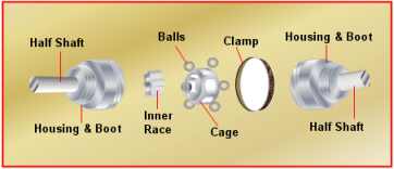
Figure 3. A CONSTANT_VELOCITY JointThe detail in the constant velocity joint is abstracted away; all intermediate parts are ignored and the input-output relationship between the shafts is captured via a simple set of algebraic constraints. Energy loss is not modeled.
- TYPE = "CYLINDRICAL"
The cylindrical joint allows two degrees of freedom between the bodies it constraints. Figure 4 shows a schematic of a cylindrical joint. It allows a body (Body-1) to translate and rotate along a fixed axis defined on another body (Body-2).

Figure 4. A CYLINDRICAL Joint - TYPE = "FIXED"
The fixed joint forces two bodies to move together as if they were welded together. No relative motion between the two bodies is allowed. Figure 5 shows a schematic of a fixed joint.

Figure 5. A Schematic of a FIXED JointThe location and orientation of any coordinate system "etched" on Body-2 is fixed with respect to any coordinate "etched" on Body-1.
- TYPE = "FREE"
The free joint is the exact opposite of the fixed joint. It does not restrict any motion between the two bodies it connects. The free joint is typically used to define topology hierarchy, when joint (also known as relative) coordinates are used to internally represent the system.

Figure 6. A FREE JointIn a free joint, any coordinate system fixed on Body-2 can move in all possible ways with respect to a coordinate system fixed on Body-1.
- TYPE = "HOOKE"The image below shows a schematic of a HOOKE joint. This joint constrains two Reference_Markers, I on Body-1 and J on Body-2 such that (a) their origins Oi and Oj remain superposed, and (b) the I marker x-axis is always perpendicular to the J marker y-axis.
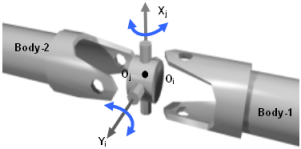
Figure 7. A HOOKE JointThe HOOKE joint removes four degrees of freedom from a system. Body-1 can rotate about the Xi axis and Body-2 can rotate about the Yi axis. Relative translations are not allowed. Physically, the HOOKE joint is identical to the UNIVERSAL joint.
- TYPE = "INLINE"
This is a constraint primitive that requires that the origin of a Reference_Marker on Body-1 translate along the z-axis of a Reference_Marker placed on Body-2. All rotations are allowed. Figure 8 shows a schematic of an INLINE primitive.

Figure 8. A Schematic of an INLINE JointThe inline primitive constrains two translational degrees of freedom. It prohibits translation along the x- and y-axes of the Reference_Marker on Body-2.
- TYPE = "INPLANE"
This is a constraint primitive that requires that the origin of a Reference_Marker on Body-1 (I in the figure below) to stay in the XY plane defined by the origin of the J Reference_Marker and its z-axis. Figure 9 shows a schematic of an INPLANE primitive.

Figure 9. A Schematic of an INPLANE JointThe INPLANE primitive constrains one translational degree of freedom. It prohibits translation along the z-axis of the Reference_Marker J on Body-2. All rotations are allowed.
- TYPE = "ORIENTATION"
Figure 10 shows a schematic of an ORIENTATION joint. It requires that the orientation of a Reference_Marker on Body-1 (I in the figure below) always be the same as the orientation of a Reference_Marker on Body-2 (J in the figure below).

Figure 10. An ORIENTATION JointThe ORIENTATION joint removes three degrees of freedom; all of these are rotational. All three translations of Body-1 with respect to Body-2 are allowed.
- TYPE = "PARALLEL_AXES"
Figure 11 shows a schematic of a PARALLEL_AXES joint. This joint constrains Body-1 such that the z-axis of a Reference_Marker (I in the figure) is always parallel to the z-axis of a Reference_Marker on Body-2 (J in the figure).

Figure 11. A PARALLEL_AXES JointThe PARALLEL_AXIS joint removes two rotational degrees of freedom. Rotation of Body-1 is only allowed about the z-axis of the I Reference_Marker. All three translations are allowed.
- TYPE = "PERPENDICULAR"
Figure 12 shows a schematic of a PERPENDICULAR_AXES joint. This joint constrains Body-1 such that the z-axis of a Reference_Marker (I in the figure) is always PERPENDICULAR to the z-axis of a Reference_Marker on Body-2 (J in the figure).

Figure 12. A PERPENDICULAR_AXES JointThe PERPENDICULAR _AXIS joint removes one degree of freedom. Rotation of Body-1 is only allowed about the z-axis of the I Reference_Marker and the z-axis of the J Reference_Marker. All three translations are allowed.
- TYPE = "PLANAR"
The planar joint requires that a Reference_Marker, I, defined on Body-1 be restricted in its movement such that its origin lies in the x-y plane defined by the origin of a Reference_Marker, J, defined on BODY-2. Figure 13 shows a schematic of a PLANAR joint.
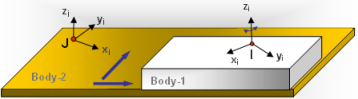
Figure 13. A Schematic of a PLANAR JointThe PLANAR joint allows three degrees of freedom, two translational degrees of freedom in the plane and one "drilling" rotational degree of freedom.
- TYPE = "RACK_PINION"
Figure 14 below depicts a rack and pinion joint. The pinion gear P is connected to the housing (not shown) such that it is allowed to rotate about an axis coming out the plane of the paper. The rack R slides from left-to-right. The RACK_PINION joint relates the rotation of the pinion θp to the translation of the rack S.

Figure 14. A RACK_PINION JointThe RACK_PINION joint allows five degrees of freedom. It imposes only one constraint on the system.
- TYPE = "REVOLUTE"
Figure 15 shows a schematic of a REVOLUTE joint. This joint constrains two Reference_Markers I and J such that (a) their origins are always superposed, and (b) their z-axes are collinear.
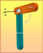
Figure 15. A REVOLUTE JointThe REVOLUTE joint removes five degrees of freedom from a system. Rotation about the common z-axes is the only motion that is allowed.
- TYPE = "SCREW"
Figure 16 depicts a screw joint. Body-2 contains screw-threads with a pitch p. The axis of the screw is defined by the z-axis of a Reference_Marker J on Body-2. Body-1 has corresponding threads that allow it to mate with the threads on Body-2. A rotation of Body-2 along the screw axis causes Body-1 to translate up or down along the screw axis. The SCREW joint relates the rotation of the Body-1 about the screw axis to its translation along the screw axis.
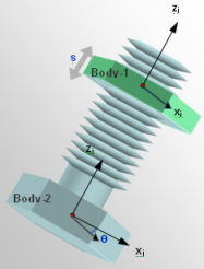
Figure 16. A SCREW JointThe SCREW joint removes only one degree of freedom from a system.
- TYPE = "SPHERICAL"
A SPHERICAL joint shows a schematic of a SPHERICAL joint. This joint constrains two Reference_Markers, I on Body-1 and J on Body-2, such that their origins Oi and Oj are always superposed.

Figure 17. A SPHERICAL JointThe SPHERICAL joint removes three degrees of freedom from a system. Body-2 is allowed to rotate with respect to Body-1. Relative translation is not allowed.
- TYPE = "TRANSLATIONAL"
Figure 18 shows a schematic of a TRANSLATIONAL joint. This joint constrains two Reference_Markers I and J such that (a) their orientations remain the same, and (b) they share a single common axis of translation which is the z-axis of Reference_Marker J.
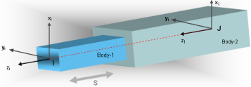
Figure 18. A TRANSLATIONAL JointThe TRANSLATIONAL joint removes five degrees of freedom from a system. Relative translation along the z-axis of Reference_Marker J is the only motion that is allowed.
- TYPE = "UNIVERSAL"
Figure 19 below shows a schematic of a UNIVERSAL joint. This joint constrains two Reference_Markers, I on Body-1 and J on Body-2 such that (a) their origins Oi and Oj remain superposed and (b) their z-axes are always orthogonal.
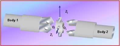
Figure 19. A UNIVERSAL JointThe UNIVERSAL joint removes four degrees of freedom from a system. Body-2 can rotate about the Zj axis and Body-1 can rotate about the Zi axis. Relative translations are not allowed.
Note that the output angular velocity will not be equal to the input angular velocity.
Let:- ù be the speed of the input shaft
- ù2 be the speed of the output shaft,
- â the angle between the shafts
- f1 the rotation angle of the input shaft
Then:
(1)
At β=π/2, the output angular velocity is zero. Physically, the shafts lock. This manifests itself as a singular matrix in MotionSolve.
Only at β=0, is the output shaft angular velocity equal to the input shaft angular velocity.
The angular acceleration of the output shaft, α2, can be expressed as:(2) - In Multibody Dynamics, a regular, or ideal
joint, can be defined as a set of algebraic constraint equations:
with q being the generalized coordinates of the system, such as the positions and orientations of each rigid body. This set of constraint equations is then incorporated into the equations of motion (EOM) in MotionSolve, using the method of Lagrange multipliers, to form a set of differential algebraic equations (DAE). Each constraint equation reduces the degrees of freedom (DOF) of the multibody system by one. The total kinematic DOFs of the mechanism will be the number of the generalized coordinates, q, minus the number of the algebraic constraint equations of the multibody system. If we virtualize the joint, the constraint equations are extended to:
with ε being treated as extra generalized coordinates and solved alongside other generalized coordinates q in the DAE. Instead of solving the algebraic equation alongside the EOM, you can instead introduce a violation force that acts in the opposite direction to the violation in order to minimize ε . The force is defined as:
where G is a gigantic factor (usually in the order of 1e12) and K is an arbitrary stiffness (for example K = 1). This equation resembles closely a second order system, such as a mass-spring-damper, where the damping factor is chosen to allow for critical damping. The precise values of G and K are intrinsic to the solver and are adjusted automatically based on the overall properties of the system and cannot be changed manually. The force f is then added to the RHS of the Equations of Motion.
The difference of this gigantic element approach compared to a general penalty approach (see bushings) lies in the degree of violation or penalty. In this novel approach, ε is kept so small that the constraint violation is in many cases undetectable without creating a large burden (numerical stiffness) for the solver. From a user’s perspective, a regular and virtual joint/constraint will provide the same kinematics and dynamics, with the exception that a virtual joint/constraint cannot introduce constraint redundancy. Furthermore, virtual joints/constraints can be thought of as “soft coupling” that allows for other numerical approaches to solve the General Equations of Motions.
Virtual constraints can be used in all analysis types, such as static, quasi-static, transient, and linear. As their algebraic counterpart, they can be activated and deactivated within an analysis.