Evaluation of iron and magnetic losses with a hysteretic material characterized by a Preisach model
Introduction
This chapter deals with the evaluation of iron and hysteretic losses with a material characterized by a Preisach model of the following types:- Isotropic hysteretic, Preisach model described by 4 parameters of a typical cycle and
- Isotropic hysteretic, Preisach model identified by N triplets.
The materials having this type of B(H) property take into account ferromagnetic hysteresis phenomena during the resolution of the project. Therefore, they allow a direct or a priori evaluation of iron and hysteretic losses in the ferromagnetic material.
The following subjects are covered in the next three sections:
- Static and dynamic hysteresis ;
- Consideration of iron and hysteretic losses in Flux for a hysteretic material;
- Application example
Static and dynamic hysteresis
During the operation of electromechanical devices, their parts are subjected to time-varying magnetic fields. These induce eddy currents (also called Foucalt currents) in the volumes of the conducting parts that result in losses via the Joule effect. Furthermore, in the parts composed by ferromagnetic materials exhibiting a hysteretic behavior, variations of the magnetic field also generate losses related to the successive magnetization and demagnetization processes.
In such devices, the total power dissipated at a point of the magnetic material (usually referred to as iron losses in the context of electromechanics) and may be written as follows:
(1)
With
- p: the density of iron losses (W/m³) ;
- H : the magnetic field (A/m) ;
- B : the magnetic induction (T) ;
- ρ: the electrical resistivity of the material (Ω.m) ;
- J: the induced current density (A/m²).
While expression (1) is valid at each point of the magnetic material, a similar expression may be derived for a volume region through its integration and written in terms of measurable macroscopic quantities (further details in the bibliographical references at the end of this chapter). Indeed, the total power density absorbed in such a region (i.e., the total iron losses, including both hysteretical losses and Joule losses) is given simply by
(2)
in which now
- P is the iron losses density in the region (W/m³) ;
- Hs is the surface magnetic field on the region (A/m) and
- Ba is the average magnetic induction in the cross section of the region (T).
In (1), two terms may be clearly distinguished. The first contribution is directly related to the magnetization state of the material and corresponds to the the time rate of change of the energy stored in the magnetic field in the material. The second term is related to the eddy currents induced in the conducting medium and represent the Joule losses. In the case of slowly varying fields, the Joule losses term is small because the induced currents are negligible and the losses are almost purely hysteretical in nature. On the other hand, when the time rate of change of the fields increases, both the hysteretical losses and Joule losses tend to increase.
Equation (2) on the other hand contains only a single term on its right hand side, which accounts for both hysteretical and eddy current losses. This term could be mistakenly considered a purely hysteretic loss term when compared to equation (1), but this is not the case. Indeed, since Hs and Ba are functions of the overall distribution of fields in the region (including the contribution arising from eddy currents at higher frequencies), the term Hs*dBa/dt accounts for the complete iron losses in the volume region.
It follows from the above that the area enclosed by the hysteresis cycle of Ba(Hs) represents the total energy dissipated in a cycle (i.e. the sum of both hysteretical and Joule losses). At low frequencies, the hysteresis cycle is narrow due to negligible induced currents and Joule losses. Under these circumstances, we speak of static hysteresis. At higher frequencies, the hysteresis cycle Ba(Hs) widens due to the development of induced currents leading to Joule losses and we are now speaking about dynamical hysteresis . These effects are illustrated in th figure below:

Figure 1. Static hysteresis cycle (at 10 Hz, in red) and dynamical hysteresis cycle (at 1000Hz, in blue) in a magnetic region subjected to eddy currents.
Evaluating iron and magnetic losses in Flux with a hysteretic material
In a Flux project containing a Transient magnetic application, the user may choose between two approaches to evaluate iron losses losses during the resolution:
- To represent static hysteresis only, a material containing a hysteretic B(H) property based on the Preisach model must be defined and assigned to a magnetic non-conducting region. This approach is well-adapted for low frequency problems.
- To represent dynamic hysteresis, i.e. to evaluate increased iron losses due to eddy currents, the material containing a Preisach B(H) property must also include a J(E) property and be assigned to a solid conductor region instead of a non-conducting magnetic region.
- Create a Sensor of type Predefined;
- In the predefined quantities, choose Magnetic power;
- Select the non-conductive magnetic regions with a hysteretic B(H) property.This
predefined sensor evaluates the following expression which represents
dissipated power density associated to static hysteresis:
This expression may also be evaluated through the quantity dPowMag/dV available in the formula editor. Its spatial distribution may also be visualized through an isovalues plot in post-processing.
In the second case (i.e. dynamic hysteresis: material with both properties J(E) and Preisach B(H) and solid conductor region), the user must
- Create a Sensor of type Integral;
- Select the solid conductor region containing the hysteretic property B(H) and a conductivity model J(E) ;
- In tthe field Spatial formula, select the quantity dPower/dV in the formula
editor. This quantity calculates the following expression and allows the iron
losses to be fully taken into account:
The distribution of iron losses in the device may also be visualized in the isovaleurs using the quantity dPower/dV.
The table below summarizes the two modeling approaches described in this section.
| Material | Active property | Region | Computation method | Evaluated quantity |
|---|---|---|---|---|
| Hysteretic Isotropic Material characterized by a Preisach-type model | B(H) | Magnetic non-conducting | Predefined sensor (type magnetic power) on a region (quantity dPowMag/dV) |
Magnetic power
|
| B(H) and J(E) | Solid Conductor | Sensor evaluating the integral of quantity dPower/dV on a region. | Iron losses
|
Application example
- the static hysteresis approach: based on a material containing a Preisach B(H) property assigned to a magnetic non-conducting region.
- the dynamical hysteresis approach: based upon a material containing both a Preisach B(H) property and a J(E) property assigned to a solid conductor region.
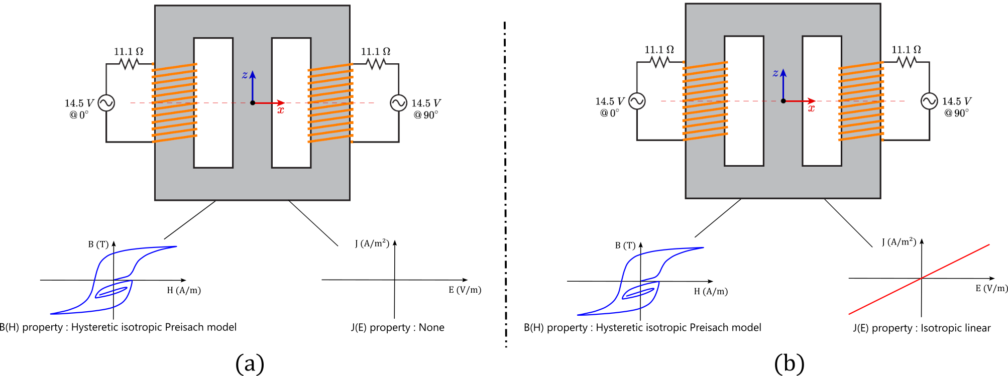
Figure 2. 2D representation of Problem TEAM 32 with (a) the approach with a non-conducting magnetic region and a hysteretic B(H) property and (b) the approach with a bulk conductor-like region, a hysteretic B(H) property, and an isotropic linear J(E) property.
The two voltage sources that feed the circuit impose a sinusoidal voltage with an amplitude of 14.5 V and a phase shift of 90°. Several computations were performed, with the frequency of the voltage sources going from 1 to 100Hz and with both approaches. The goal is to compare the instantaneous hysteretical losses with the total iron losses for each frequency.
After resolution, a comparison between the two previous approaches may be performed by comparing the total iron losses with the hysteretic losses, as shown in the figure below:

Figure 3. The total power dissipated in the magnetic core as a function of the supply frequency. The orange line corresponds to the approach based on a non-conducting magnetic region and a material with hysteretic B(H) property. The blue line on the other hand corresponds to the approach using a solid conductor region and a material with hysteretic B(H) and linear isotropic J(E) properties.
The eddy current distribution may be visualized trough an arrow plot of the current density J in the magnetic core, as shown in the figure below.

Figure 4. Distribution of induced currents evolving in the volume of the magnetic core evaluated with the approach based on a solid conductor region, a hysteretic B(H) property and an isotropic linear J(E) property.
Bibliographical references
- H. Pfützner and G. Shilyashki, "Theoretical Basis for Physically Correct Measurement and Interpretation of Magnetic Energy Losses," in IEEE Transactions on Magnetics, vol. 54, no. 4, pp. 1-7, April 2018, Art no. 6300207, doi: 10.1109/TMAG.2017.2782218.
- M. Tousignant. Modélisation de l’hystérésis et des courants de Foucault dans les circuits magnétiques par la méthode des éléments finis. Energie électrique. Université Grenoble Alpes; Polytechnique Montréal (Québec, Canada), 2019. (in French). ⟨NNT : 2019GREAT065⟩. ⟨tel-02905410⟩