Random Response Analysis
Used when a structure is subjected to a non-deterministic, continuous excitation.
Cases likely to involve non-deterministic loads are those linked to conditions such as turbulence on an airplane structure, road surface imperfections on a car structure, noise loads on a given structure, and so forth.
Random Response Analysis requires as input, the complex frequency responses from Frequency Response Analysis and Power Spectral Density Functions of the non-deterministic Excitation Source(s). The Complex Frequency Responses can be generated by Direct or Modal Frequency Response Analysis.
Different Load Cases (a and b)
Where, is the cross power spectral density of two (different, ) sources, where the individual source is the excited load case and is the applied load case. This value can possibly be a complex number. is the complex conjugate of .
Same Load Case (a)
Combination of Different (a,b) and Same (a,a) Load Cases in a Single Random Response Analysis
If there is a combination of load cases for Random Response Analysis, the total power spectral density of the response will be the summation of the power spectral density of responses due to all individual (same) load cases as well as all cross (different) load cases.
Auto-correlation Function
- The time lag for Auto-correlation
RMS of the Response Power Spectral Densities for degree of freedom "x"

Figure 1.
Auto-correlation Function Output for degree of freedom "x"
The RANDT1 Bulk Data Entry can be used to specify the lag time () used in the calculation of the Auto-correlation function for each response for a particular degree of freedom, .
The Auto-correlation Function is calculated for each time lag value in the specified RANDT1 set over the entire frequency range [0, ].
Number of Positive Zero Crossing
If XYPLOT, XYPEAK or XYPUNCH, output requests are used, the root mean square value and the maximum number of positive crossing calculated at each excitation frequency will be exported to the *.peak file.
Setup
Random response analysis is activated, for a particular subcase, through the inclusion of the RANDOM Subcase Information Entry in the Subcase, along with the optional ANALYSIS=RANDOM entry.
This selector identifies RANDPS and the optional RANDT1 Bulk Data Entries to be used for random response analysis. The complex frequency responses and input spectral density is specified by the RANDPS Bulk Data Entry. The RANDPS data refers to a TABRND1 Bulk Data Entry, which contains the power spectral density of the loading versus frequency. The RANDT1 Bulk Data Entry describes the time span for the auto-correlation. The RCROSS Bulk Data Entry is used to request the output of the cross-power spectral density function for Random Response Analysis and is referred to by the RCROSS I/O Options Entry section selector. Loading for each frequency response subcase may be distinct, but all frequency response subcases referenced in a particular Random Subcase should reference the same frequency data.
The RANDT1 Bulk Data Entry describes the time lag set for the calculation of the Auto-correlation function. The RCROSS Bulk Data Entry is used to request the output of the cross power spectral density function for specific responses from the Random Response Analysis and is referred to by the RCROSS I/O Options Entry selector. Loading for each frequency response subcase may be distinct, but frequency response subcases referenced in a particular Random Subcase should reference the same frequency data.
Random Response analysis can also be conducted based on Frequency Response results from a preexisting H3D file.
Frequency response results such as DISPLACEMENT, VELOCITY and ACCELERATION from the H3D file can be imported to the random response analysis. In this process, if FORCE / ELFORCE of 1D/2D elements, STRESS / ELSTRESS, STRAIN or Energy output (ESE/EKE/EDE) is requested in random response analysis, then the preexisting H3D file must have either of rotational displacement, rotational velocity or rotational acceleration results. This is also the case when rotational result (displacement, velocity or acceleration) output is requested in the Random Response Analysis.
The IMPORT I/O Entry and the ASSIGN,H3DRES entry are available to identify such H3D files and the corresponding subcase whose results are to be used for subsequent Random Response Analysis.

Figure 2.
Results Output
The Random Response Power Spectral Density Function (PSDF) can be written to the .h3d file for DISP, VELO, and ACCE using the PSDF output option on these I/O Option data selectors within the Random Subcase.
At the end of the output for all the frequencies is the RMS over frequencies output selector in HyperView, as shown below.
The Random Response Power Spectral Density Function (PSDF) can be written to the .h3d file for CBUSH element forces using the FORCE I/O Options Entry by specifying the PSDF output option within the Random Subcase. At the end of the output for each frequency is the RMS over frequencies output selector for the .h3d file in HyperView, as shown below.
The Random Response Power Spectral Density Function (PSDF) can be written to the .h3d and .op2 files for solid and shell elements for stress and strain with the STRESS and STRAIN I/O Options using the PSDF output option within the Random Subcase. At the end of the output for each frequency is the RMS over frequencies output selector for the .h3d file and the Simulation selector for the .op2 file in HyperView, as shown below.
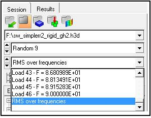
Figure 3. RMS Output Selection in H3D File in HyperView
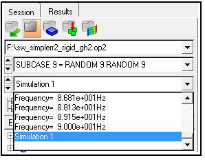
Figure 4. RMS Output Selection in OP2 File in HyperView
Plot Output
Three plotting output requests may be used for random response analysis results.
- Plotting Controllers
- XYPEAK
- Generates a .peak file containing a summary of the requested output
- XYPLOT
- Generates a HyperGraph session file (_rand.mvw file) and related data file (.rand file) for the requested output. Also generates the .peak file.
- XYPUNCH
- Generates a .pch file for the requested output. Also generates the .peak file.
These output requests are different from most other OptiStruct output requests in that they may be combined on the same line.
- "Operation" can be any combination of XYPLOT, XYPUNCH, and XYPEAK.
- "Curve-type" can be FORCE, STRESS, STRAIN, DISP, VELO, or ACCE to request force, stress, strain, displacement, velocity or acceleration, respectively.
- "Plot-type" can be either PSDF or AUTO to request power spectral density function or auto-correlation, respectively.
- "Grid (Component) list" must come after a slash "/". Each entry in the list is comma separated. Each entry consists of a GRID or SPOINT ID followed by a component of motion (T1, T2, T3, R1, R2, or R3) in parentheses. For SPOINTs the component must be T1.
In addition, plot titles and axis labels may be controlled using TCURVE (plot title), XTITLE (x-axis label), and YTITLE (y-axis label). Default titles and labels are generated when these controls are not used.
Example Results
Example: Results in HyperGraph
XYPLOT, VELO, PSDF / 3(T2), 6(T2)Example: Results in .peak file
XYPEAK,DISP, AUTO /223(T3)Example: Results in all Formats
Requesting random response results output, in all formats, for the acceleration PSDF for GRIDS 8 and 9 for components T1 and T2:
XYPEAK, XYPLOT, XYPUNCH, ACCE, PSDF / 8(T1), 9(T1), 8(T2), 9(T2)Here the XYPEAK request is valid, but redundant as it is always created when XYPLOT or XYPUNCH is present.