Gradient-based Optimization Method
The following features can be found in this section:
Iterative Solution
- Analysis of the physical problem using finite elements.
- Convergence test; whether or not the convergence is achieved.
- Response screening to retain potentially active responses for the current iteration.
- Design sensitivity analysis for retained responses.
- Optimization of an explicit approximate problem formulated using the sensitivity information. Back to step 1.
To achieve a stable convergence, design variable changes during each iteration are limited to a narrow range within their bounds, called move limits. The biggest design variable changes occur within the first few iterations and, due to an advanced formulation and other stabilizing measures, convergence for practical applications is typically reached with only a small number of FE analyses.
The design sensitivity analysis calculates derivatives of structural responses with respect to the design variables. This is one of the most important ingredients for taking FEA from a simple design validation tool to an automated design optimization framework.
The design update is generated by solving the explicit approximate optimization problem, based on sensitivity information. OptiStruct has two classes of optimization methods implemented: dual method and primal method. The dual method solves the optimization problem in the dual space of Largrange multipliers associated with active constraints. It is highly efficient for design problems involving a very large number of design variables but much fewer constraints (common to topology and topography optimization). The primal method searches the optimum in the original design variable space. It is used for problems that involve equally as many design constraints as design variables, which is common for size and shape optimizations. The choice of optimizer is made automatically by OptiStruct, based on the characteristics of the optimization problem.
Regular or Soft Convergence
Two convergence tests are used in OptiStruct and satisfaction of only one of these tests is required.
Regular convergence (design is feasible) is achieved when the convergence criteria are satisfied for two consecutive iterations. This means that for two consecutive iterations, the change in the objective function is less than the objective tolerance and constraint violations are less than 1%. At least three analyses are required for regular convergence, as the convergence is based on the comparison of true objective values (values obtained from an analysis at the latest design point). An exception (design is infeasible) is when the constraints remain violated by more than 1%, and for three consecutive iterations the change in the objective function is less than the objective tolerance and the change in the constraint violations is less than 0.2%. In this case, the iterative process will be terminated with a conclusion 'No feasible design can be obtained.'
Soft convergence is achieved when there is little or no change in the design variables for two consecutive iterations. It is not necessary to evaluate the objective (or constraints) for the final design point, as the model is unchanged from the previous iteration. Therefore, soft convergence requires one less iteration than regular convergence.
Optimization Algorithms
OptiStruct utilizes gradient-based optimization algorithms to solve the optimization problem.
- Method of Feasible Directions (MFD)
- Sequential Quadratic Programming (SQP)
- Dual Optimizer based on separable convex approximation (DUAL)
- Enhanced Dual Optimizer based on separable convex approximation (DUAL2)
- Large scale optimization algorithm (BIGOPT)
- Method of Moving Asymptotes (MMA)
MFD, SQP, DUAL, and DUAL2 are standard optimization algorithms. For further information, refer to relevant books and papers in the References section. Refer to the section below for more information on BIGOPT.
During a run, the corresponding optimization algorithms are automatically selected by OptiStruct based on the optimization type. The DOPTPRM, OPTMETH parameter can be used to change the default optimization algorithms. The use of this parameter will override the defaults.
DUAL2 is an enhanced version of the proprietary CONLIN dual optimizer. Solution stability has been improved, reducing probability of failure in converging to a solution. The default optimizer for problems with a large number of design variables such as topology, free-size and topography is DUAL2. You can switch to DUAL or MMA in case you run into issues with the default DUAL2 method fails to converge for Topology, Free-Size, or Topography optimization.
MFD is the default optimizer for problems with a large number of constraints (but smaller number of design variables) such as size/gauge and shape.
MFD, SQP (primal methods) and BIGOPT are more suitable for size/gauge and shape since the approximate problem typically involves coupled terms, due to the advanced approximation formulation utilizing intermediate variables and responses.
If Equality Constraints are activated in size and shape optimization, then SQP is the default optimizer.
DOPTPRM,OPTIMOMP,YES can be used to turn on parallel computation for MFD, SQP, and DUAL2 algorithms.
Large Scale Optimization Algorithm (BIGOPT)
A gradient-based method that consumes less memory and is relatively more computationally efficient, compared to MFD and SQP.
Implementation
Where, is the objective function, is the i’th constraint function, is the number of equality constraints, is the total number of constraints, is the design variable vector, and and are the lower and upper bound vectors of design variables, respectively.
Where, and are penalty multipliers.
BIGOPT considers the bound constraints separately. So the original problem is converted to an unconstrained problem. Polak-Ribiere conjugate gradient method is used to generate search direction. After the search direction is calculated, a one-dimensional search can be accomplished by parabolic interpolation (Brent’s method).
Terminating Conditions
- and the design is feasible.
- and the design is feasible.
- The number of iteration steps exceeds .
Where, is the gradient of , is the ’th iteration step, is the convergence parameter, and is the allowed maximum iterations.
Sensitivity Analysis
Using this equation, the largest cost in the calculation of the response gradient is the forward-backward substitution required for the calculation of the derivative of the displacement vector with respect to the design variable. This is called the direct method. One forward-backward substitution is required for each design variable.
If constraints are active in more than one load case, and the load is a function of the design variable (say body force or pressure loads for shape optimization), then the set of forward-backward substitutions must be performed for each active load case. If the loads are not a function of the design variables, but there are active load cases with multiple boundary conditions, then the set of forward-backward substitutions must be performed for each active boundary condition.
When the adjoint variable method for sensitivity analysis is used, a single forward-backward substitution is needed for each retained constraint. This forward-backward substitution is needed to calculate the vector .
There are typically a small number of design variables in shape and size optimization (say 5 to 50) and a large number of constraints. The large number of constraints comes from stress constraints. If there are 20,000 elements, each with a single stress constraint, and 10 load cases, there are a total of 200,000 possible stress constraints.
There are typically a large number of design variables in topology optimization (between 1 and 3 per element) and a small number of constraints. Because stress constraints are not usually considered in topology optimization, it makes sense that the adjoint variable method of sensitivity analysis be used for topology optimization (in order to reduce computational costs).
For shape and sizing (parameter) optimization, it is often beneficial to use the direct method for sensitivity analysis. However, in some cases, when there are a large number of design variables and a small number of constraints, the adjoint variable method should be used. For example, in a topography optimization, the number of constraints that gradients need to be calculated for can be reduced using constraint screening. With constraint screening, constraints that are not close to being violated are ignored. Only constraints that are violated, or nearly violated, are retained. Also, if there are many stress constraints that are retained in a small region of the structure, say at a stress concentration, only a few of the most critical need to be retained.
The sensitivities of responses with respect to design variables can be exported to an Excel spreadsheet (OUTPUT,MSSENS) or plotted in HyperGraph (OUTPUT,HGSENS). For contouring in HyperView, the sensitivities of topology, free-sizing and gauge design variables can be exported to H3D format (OUTPUT,H3DTOPOL and OUTPUT,H3DGAUGE, respectively). Sensitivity output in ASCII format for topology and free-sizing variables can be requested through OUTPUT,ASCSENS.

Figure 1. Input File of DOPTPRM,DESMAX,0 and OUTPUT,H3DTOPOL in Sensitivity Analysis
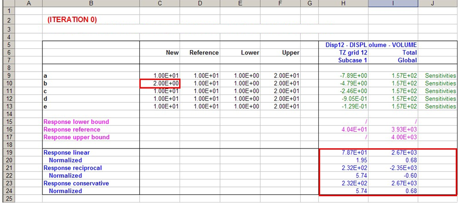
Figure 2. Output Showing Modification (Field C10) Yields Approximate Results (Lower Right)
Move Limit Adjustments
Move limits on the design variables, and/or intermediate design variables, are used to protect the accuracy of the approximations.
Small move limits lead to smoother convergence. Many iterations may be required due to the small design changes at each iteration. Large move limits may lead to oscillations between infeasible designs as critical constraints are calculated inaccurately. If the approximations themselves are accurate, large move limits can be used. Typical move limits in the approximate optimization problem are 20% of the current design variable value. If advanced approximation concepts are used, move limits up to 50% are possible.
Even with advanced approximation concepts, it is possible to have poor approximations of the actual response behavior with respect to the design variables. It is best to use larger move limits for accurate approximations and smaller move limits for those that are not so accurate.
The same set of design variable move limits must be used for all of the response approximations. It is important to look at the approximations of the responses that are driving the design. These are the objective function and most critical constraints. If the objective function moves in the wrong direction, or critical constraints become even more violated, it is a sign that the approximations are not accurate. In this case, all of the design variable move limits are reduced. However, if the move limits become too small, convergence may be slowed, as design variables that are a long way from the optimum design are forced to change slowly. Therefore, the move limits on the individual design variables that keep hitting the same upper or lower move limit bound are increased. Move limits are automatically adjusted by OptiStruct.
Constraint Screening
At each iteration of the optimization process, the objective function(s) and all constraints of the design problem are evaluated.
- This can result in a big optimization problem with a large number of responses and design variables. Most optimization algorithms are designed to handle either a large number of responses or a large number of design variables, but not both.
- For gradient-based optimization, the design sensitivities of these responses need to be calculated. The design sensitivity calculation can be very computationally expensive when there are a large number of responses and a large number of design variables.
Constraint screening is the process by which the number of responses in the optimization problem is trimmed to a representative set. This set of retained responses captures the essence of the original design problem while keeping the size of the optimization problem at an acceptable level. Constraint screening utilizes the fact that constrained responses that are a long way from their bounding values (on the satisfactory side) or which are less critical (i.e. for an upper bound more negative and for a lower bound more positive) than a given number of constrained responses of the same type, within the same designated region and for the same subcase, will not affect the direction of the optimization problem and therefore can be removed from the problem for the current design iteration.
Consider the optimization problem where the objective is to minimize the mass of a finite element model composed of 100,000 elements, while keeping the elemental stresses below their associated material's yield stress. In this problem, there are 100,000 constraints (the stress for every element must be below its associated material's yield stress) for each subcase. For every design variable, 100,000 sensitivity calculations must be performed for each subcase, at every iteration. Because design variable changes are restricted by Move Limit Adjustments, stresses are not expected to change drastically from one iteration to the next. Therefore, it is wasteful to calculate the sensitivities for those elements whose stresses are considerably lower than their associated material's yield stress. Also the direction of the optimization will be driven primarily by the highest elemental stresses. Therefore, the number of required calculations can be further reduced by only considering an arbitrary number of the highest elemental stresses.
Of course there is trade-off involved in using constraint screening. By not considering all of the constrained responses, it may take more iterations to reach a converged solution. If too many constrained responses are screened, it may take considerably longer to reach a converged solution or, in the worst case, it may not be able to converge on a solution if the number of retained responses is less than the number of active constraints for the given problem.
Through extensive testing it has been found that, for the majority of problems, using constraint screening saves a lot of time and computational effort. Therefore, constraint screening is active in OptiStruct by default. The default settings consider only the 20 most critical (that is, for an upper bound most positive and for a lower bound most negative) constraints that come within 50 percent of their bound value (on the satisfactory side) for each response type, for each region, for each subcase.
The DSCREEN Bulk Data Entry controls both the screening threshold and number of retained constraints. Different DSCREEN settings are allowed for all of the response types supported by the DRESP1 Bulk Data Entry. Responses defined by the DRESP2 Bulk Data Entry are controlled by a single DSCREEN entry with RTYPE=EQUA. Likewise, responses defined by the DRESP3 Bulk Data Entry are controlled by a single DSCREEN entry with RTYPE=EXTERNAL. It is important to ensure that DRESP2 and DRESP3 definitions that use the same region identifier use similar equations. (In order for constraint screening to work effectively, responses within the same region should be of similar magnitudes and demonstrate similar sensitivities, the easiest way to ensure that is through the use of similar variable combinations).
It is possible to allow the screening criteria to be automatically and adaptively adjusted in an effort to retain the least number of responses necessary for stable convergence. Setting the second field as AUTO on the alternate format of the DSCREEN Bulk Data Entry will enable this feature. Region definition is also automated with this setting. This setting is useful for less experienced users and can be particularly useful when there are many local constraints. However, there are some drawbacks; experienced users may be able to achieve better performance through manual definition of screening criteria, more memory may be required to run with AUTO, and manual under-retention of constraints will require less memory and may; therefore, be desirable for very large problems (even with compromised convergence stability and optimality). Five levels of automatic screening (AUTO) are available via the LEVEL field. To turn OFF automatic screening completely, set the LEVEL field to OFF.
- DOPTPRM,GBUCK,1 will be turned on if it is not specified by you and the lowest 15 buckling modes will be considered in optimization. This helps improve the stability of convergence. Constraining only the lowest or a few buckling eigenvalues will lead to unstable convergence as the buckling modes could change from iteration to iteration, which also means the retained buckling modes could change. The better formulation would be to constrain the lowest 10 to 15 modes (or more, depending on how many modes come close to the bound).
- The upper bound on the EIGRL card will be adjusted in order to calculate only the buckling eigenvalues, which are potentially retained in optimization. To improve performance, OptiStruct will try to avoid calculating buckling eigenvalues which are far away from the bound (that is, in the safe zone).
Automatic screening (including buckling adjustments mentioned above) can be completely disabled by setting DCREEN,AUTO,OFF. However, if only the automatic screening for buckling is to be disabled (which may be required when you want to retain automatic screening for local responses, such as Stress), then the NOBUCK option can be specified on the BUCK (fourth) field of the DSCREEN entry.
Regions and Their Purpose
In OptiStruct, a region is a group of responses of the same type.
Regions are defined by the region identifier field on the DRESP1, DRESP2, and DRESP3 Bulk Data Entries used to define the responses. If the region identifier field is left blank, then each property associated with the response forms its own region. The same region identifier may be used for responses of different types, but remember that because they are not of the same type they cannot form the same region.
Example 1
| (1) | (2) | (3) | (4) | (5) | (6) | (7) | (8) | (9) | (10) |
|---|---|---|---|---|---|---|---|---|---|
| DRESP1 | 1 | label | STRESS | PSHELL | SMP1 | 1 | |||
| 2 | 3 |
DRESP1 with ID 1 defines stress responses for all the elements that reference the PSHELL definitions with PID 1, 2, or 3. As no region identifier is defined, the stress responses for each PSHELL form their own regions. So, all of the stress responses for elements referencing PSHELL with PID1 are in a different region than all of the stress responses for elements referencing PSHELL with PID2, which in turn are in a different region than all of the stress responses for elements referencing PSHELL with PID3. If this response definition is constrained in an optimization problem, and the default settings for constraint screening are assumed, then 20 elemental stresses are considered for each of the three PSHELL definitions, i.e. 20 for each region, giving a total of 60 retained responses.
Example 2
| (1) | (2) | (3) | (4) | (5) | (6) | (7) | (8) | (9) | (10) |
|---|---|---|---|---|---|---|---|---|---|
| DRESP1 | 2 | label | STRESS | PSHELL | 1 | SMP1 | 1 | ||
| 2 | |||||||||
| (1) | (2) | (3) | (4) | (5) | (6) | (7) | (8) | (9) | (10) |
| DRESP1 | 3 | label | STRESS | PSHELL | 1 | SMP1 | 3 |
All of the stress responses defined in the DRESP1 entries above form a single region - notice the entries (not blank) in field 6. Now, if these response definitions which are of the same type (STRESS) with the same entry (not blank) in field 6 are constrained in an optimization problem (assuming the default settings for constraint screening), then 20 elemental stresses are considered in total for the three PSHELL definitions because they form a single region.
Discrete Design Variables
The discrete values have a continuous trend, such as when a sheet material is provided with a range of thicknesses.
OptiStruct uses a gradient-based optimization approach for size and shape optimization. This method does not work well for truly discrete design variables, such as those that would be encountered when optimizing composite stacking sequences. The adopted method works best when the discrete intervals are small. In other words, the more continuous-like the design problem behaves, the more reliable the discrete solution will be. For example, satisfactory performance should not be expected if a thickness variable is given two discrete values 0 and T.
It is known that rigorous methods such as branch and bound are very time consuming computationally. Therefore, a semi-intuitive method was developed that is targeted at solving relatively large size problems efficiently. It is recommended to benchmark the discrete design against the baseline continuous solution. This helps to quantify the trade-off due to discrete variables and to understand whether the discrete solution is reasonable. As local optima are always a barrier for none convex optimization problems, and discrete variables tend to increase the severity of this phenomenon, it could be helpful to run the same design problem from several starting points, especially when the optimality of a solution is in doubt.
It is also possible to mix these discrete variables with continuous variables in an optimization problem.
Discrete design variables are activated by referencing a DDVAL entry on a DESVAR card.
With the DDVOPT parameter on the DOPTPRM card you can choose between a fully discrete optimization or a two-phased approach where a continuous optimization is performed first, and a discrete optimization is started from the continuous optimum.
All optimization algorithms including MFD, SQP, DUAL, BIGOPT and DUAL2 support optimization problems with discrete design variables. MFD is the default approach for models with discrete design variables.