HS-4220: Size Optimization Study on an Impact Simulation Using RADIOSS
Learn how to perform a size optimization on a finite element model defined for
RADIOSS.
Before you begin, copy the model files used in
this tutorial from <hst.zip>/HS-4220/ to your working
directory.
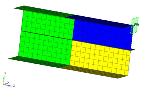
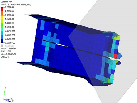
The RADIOSS model shown in Figure 1 is run using the RADIOSS Starter and Engine.
The objective is to minimize the mass of the beam under the following constraints:
Internal energy must be more than 450
Resulting reaction force must be less than 75
The input variables are the thicknesses of the four components defined in the
input deck boxbeam1._0000.rad via the /PROP/SHELL entries. They
are combined into two input variables. The thickness should be between 0.5 and 2.0;
the initial thickness is 1.0. The optimization type is size. Figure 1. Boxbeam Model, Undeformed Figure 2. Boxbeam Model, Deformed, t = 2.001
Create Base Input Template
In this step, create the base input template in HyperStudy.
Start HyperStudy.
From the menu bar, click Tools > Editor.
The Editor opens.
In the File field, navigate to your working directory and open the file
boxbeam1_0000.rad.
Create parameter for /PROP/SHELL/1.
In the Find area, enter /PROP/SHELL/1 and click
.
HyperStudy highlights /PROP/SHELL/1
in the boxbeam1_0000.rad file. Figure 3.
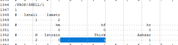
Highlight the field for thickness.
Tip: To assist you in selecting 20-character fields, press
Ctrl to activate the Selector (set to 20
characters) and then click the value. Figure 4.
Right-click on the highlighted fields and select Create
Parameter from the context menu.
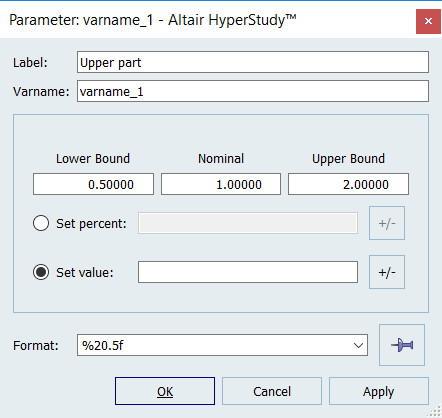
The Parameter: varname_1 dialog
opens.
In the Label field, enter Upper part.
Change bounds.
Lower Bound: 0.5
Nominal: 1.0
Upper Bound: 2.0
In the Format field, enter %20.5f.
Click OK.
Figure 5.
Assign /PROP/SHELL/2 the same thickness as /PROP/SHELL/1.
Find /PROP/SHELL/2 and highlight the field for thickness.
Right-click on the highlighted fields and select Attach to > varname_1 from the context menu.
Create parameter for /PROP/SHELL/3.
Find /PROP/SHELL/3 and highlight the field for thickness.
Right-click on the highlighted fields and select Create
Parameter from the context menu.
The Parameter: varname_2 dialog
opens.
In the Label field, enter Lower part.
Change bounds.
Lower Bound: 0.5
Nominal: 1.0
Upper Bound: 2.0
In the Format field, enter %20.5f.
Click OK.
Assign /PROP/SHELL/4 the same thickness as /PROP/SHELL/3.
Find /PROP/SHELL/4 and highlight the field for thickness.
Right-click on the highlighted fields and select Attach to > varname_2 from the context menu.
Click OK to close the Editor.
In the Save Template dialog, navigate to your working
directory and save the file as boxbeam1.tpl.
View Base Input Template in TextView
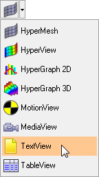
Open HyperMesh Desktop.
On the Client Selector toolbar, select TextView.
Figure 6.
Open base input template.
From the menu bar, click File > Open > Document.
In the Open Document dialog, open the
boxbeam1.tpl file.
The text editor displays the following input variables that are
defined by Templex parameter
statements:
In the Add Study dialog, enter a study name, select a
location for the study, and click OK.
Go to the Define Models step.
Add a Parameterized File model.
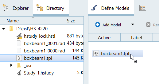
From the Directory, drag-and-drop the boxbeam1.tpl
file into the work area.
Figure 9.
In the Solver input file column, enter
boxbeam1_0000.rad.
This is the name of the solver input file HyperStudy writes during the evaluation.
In the Solver execution script column, select RADIOSS
(radioss).
Define a model dependency
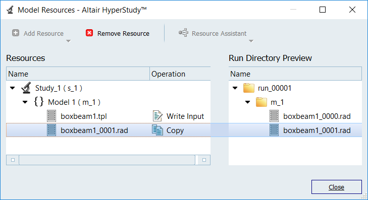
Click Model Resources.
The Model Resource dialog opens.
Select Model 1 (m_1).
Click Resource Assistant > Add File.
In the Select File dialog, navigate to your
working directory and open the boxbeam1_0001.rad
file.
Set Operation to Copy.
Click Close.
Figure 10.
Click Import Variables.
Two input variables are imported from the
boxbeam1.tpl resource file.
Go to the Define Input Variables step.
Review the input variable's lower and upper bound ranges.
Perform Nominal Run
Go to the Test Models step.
Click Run Definition.
An approaches/setup_1-def/ directory is created
inside the study Directory. The
approaches/setup_1-def/run__00001/m_1 directory
contains the input file, which is the result of the nominal run.
Create and Evaluate Output Responses
In this step you will create two output responses.
Go to the Define Output Responses step.
Create the Energy output response, which is the initial energy of the
model.
From the Directory, drag-and-drop the boxbeam1T01
file, located in
approaches/setup_1-def/run__00001/m_1, into the
work area.
In the File Assistant dialog, set the Reading
technology to Altair® HyperWorks® and click
Next.
Select Single item in a time series, then click
Next.
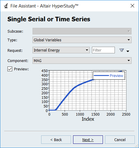
Define the following options, then click
Next.
Set Type to Global Variables.
Set Request to Internal Energy.
Set Component to MAG.
Figure 11.
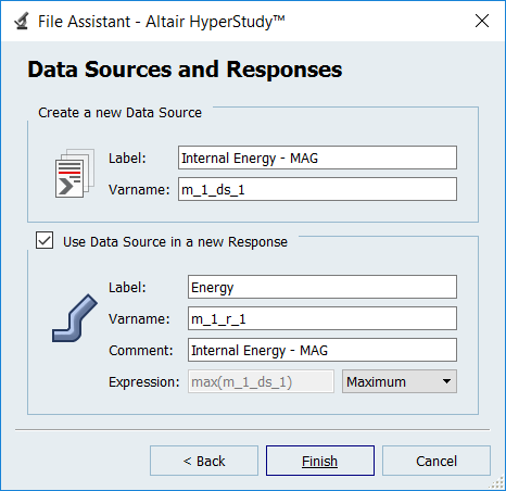
Label the output response Energy
Set Expression to Maximum.
Click Finish.
Figure 12.
Create the Force output response, which is the resultant reaction force in the
Z-direction.
From the Directory, drag-and-drop the boxbeam1T01
file, located in
approaches/setup_1-def/run__00001/m_1, into the
work area.
In the File Assistant dialog, set the Reading
technology to Altair® HyperWorks® and click
Next.
Select Single item in a time series, then click
Next.
Define the following options, then click
Next.
Set Type to Rigid wall/Wall Force.
Set Request to 1 RWALL 1.
Set Component to FNZ-Z NORMAL FORCE.
Label the output response Force
Set Expression to Maximum.
Click Finish.
Create the Mass output response.
From the Directory, drag-and-drop the boxbeam1T01
file, located in
approaches/setup_1-def/run__00001/m_1, into the
work area.
In the File Assistant dialog, set the Reading
technology to Altair® HyperWorks® and click
Next.
Select Single item in a time series, then click
Next.
Define the following options, then click
Next.
Set Type to Global Variables.
Set Request to Mass.
Set Component to MAG.
Label the output response Mass
Set Expression to First Element.
Click Finish.
Click Evaluate to extract the response values.
Run Optimization
Add an Optimization.
In the Explorer, right-click and select
Add from the context menu.
In the Add dialog, select
Optimization and click OK.
Go to the Optimization > Definition > Define Output Responses step.
Click the Objectives/Constraints - Goals tab.
Apply an objective on the Mass output response.
Click Add Goal.
In the Apply On column, select Mass.
In the Type column, select Minimize.
Figure 13.
Apply a constraint to the Energy output response.
Click Add Goal.
In the Apply On column, select Energy.
In the Type column, select Constraint.
deterministic
In column 1, select >= (less than or equal
to).
In column 2, enter 450.
Figure 14.
Apply a constraint to the Force output response.
Click Add Goal.
In the Apply On column, select Force.
In the Type column, select Constraint.
deterministic
In column 1, select <= (less than or equal
to).
In column 2, enter 75.
Go to the Optimization > Specifications step.
In the work area, set the Mode to Adaptive
Response Surface Method (ARSM).
Note: Only the methods that are valid for the problem formulation are enabled.
Click Apply.
Go to the Optimization > Evaluate step.
Click Evaluate Tasks.
Go to the Optimization > Post-Processing step.
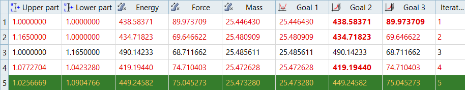
View iteration history of optimization.
Click the Iteration History tab to display data
in a tabluar view.
The optimal design is highlighted green, the infeasible designs
are shown with red text, and the violated constraints are indicated in
bold text. Figure 15.
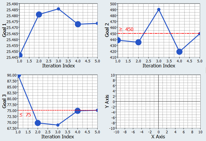
Click the Iteration Plot tab to plot the
iteration history of the study's objectives and constraints.
In the initial design, the design was infeasible as indicated by
the large circular marker for the first iteration. A view of the
constraint plots shows that the second constraint was violated in the
initial design. Initially, the optimizer added some weight in order to
satisfy the design constraints. Notice that both constraints are near
their bounds in the optimal design. Figure 16.
 .
HyperStudy highlights /PROP/SHELL/1 in the boxbeam1_0000.rad file.
.
HyperStudy highlights /PROP/SHELL/1 in the boxbeam1_0000.rad file.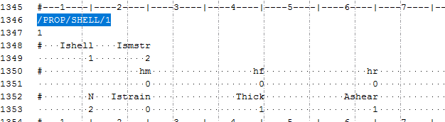
 (Find).
 .
The parameterized /PROP/SHELL cards, which reference the input variables, highlights.
.
The parameterized /PROP/SHELL cards, which reference the input variables, highlights.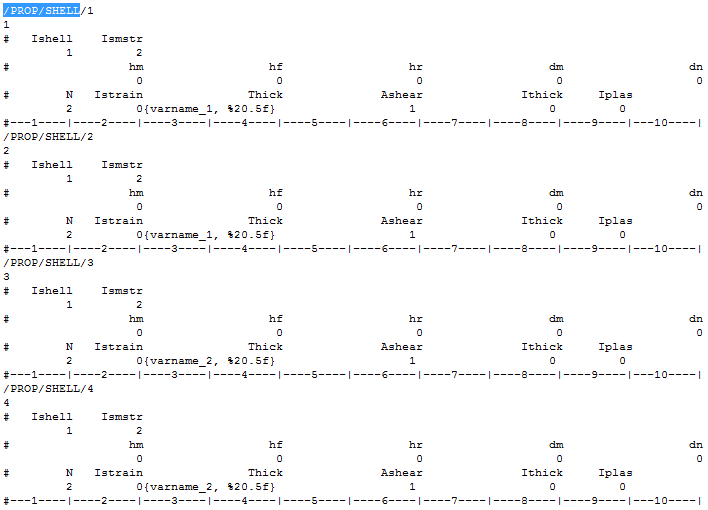
 .
The text editor evaluates the Templex statements, and replaces the parameters with their initial values.
.
The text editor evaluates the Templex statements, and replaces the parameters with their initial values.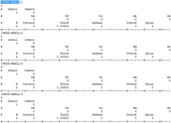
 .
.