HS-4450: Multi-Objective Optimization of a Cantilever Ibeam using an Inclusion Matrix
Learn how to use the data created from a DOE and pass it to an optimization problem via an inclusion matrix which re-uses the data.
Before you begin, copy the model files used in
this tutorial from <hst.zip>/HS-4450/ to your working
directory.
The inclusion matrix feature passes an already existing set of data to the running process. In this tutorial, the data created from a DOE is passed to an optimization problem which reuses the data. This promotes efficient design exploration practices: an optimization using a direct solver call can still be done in combination with a DOE to study the system without any loss of data. This
Perform the Study Setup
-
Start a new study in the following ways:
- From the menu bar, click .
- On the ribbon, click
 .
.
-
Add a Parameterized File model.
-
From the Directory, drag-and-drop the ibeam.tpl
file into the work area.
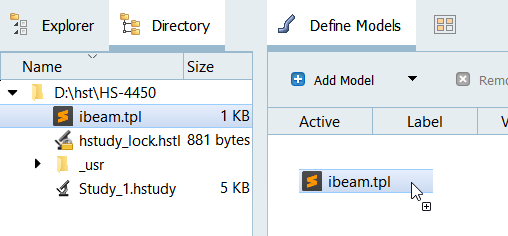
Figure 1.
-
From the Directory, drag-and-drop the ibeam.tpl
file into the work area.
Perform Nominal Run
Create and Evaluate Output Responses
-
Create the Iy output response for the y-axis moment of inertia.
-
Define the following options, then click
Next.
- Set Type to Output.
- Set Request to Iy.
- Set Component to Value.
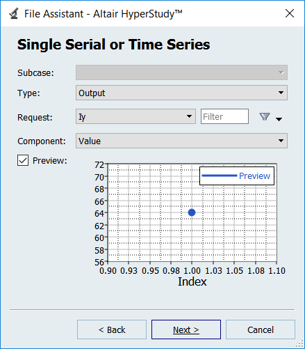
Figure 2. -
Click Finish.
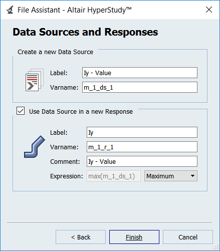
Figure 3.
-
Define the following options, then click
Next.
Run a Hammersley DOE Study
-
In the Settings tab, verify the Number of Runs is
17.
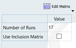
Figure 4. -
Click the Pareto Plot tab.
In the options menu, ensure that Linear effects is enabled.A Pareto Plot shows the ranked influence of the input variables on the output response. For example, for the y-axis moment of the inertia, height has the largest influence and web thickness has the least. In contrast, for the z-axis moment of inertia, the flange length and flange thickness are the most influential variables. The size of the bar indicates the magnitude of the influence, and the hashed line’s slope indicates the sign of the effect: positive or negative. For example, increasing the height will increase Iy, but it will decrease displacement.
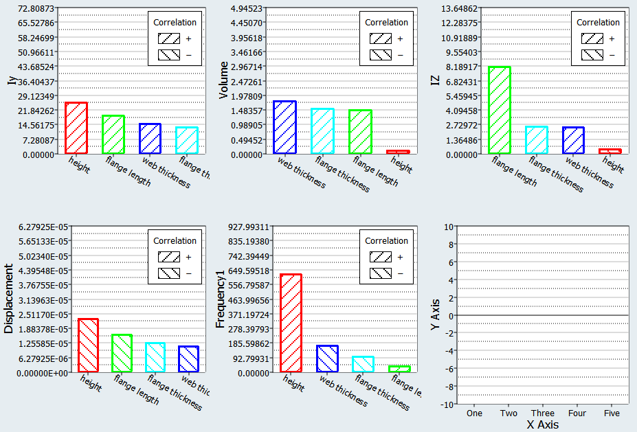
Figure 5.
Run Optimization
-
Apply an objective to the Volume output response.
- Click Add Goal.
- In the Apply On column, select Volume.
- In the Type column, select Minimize.

Figure 6. -
Apply an objective to the Iy output response.
- Click Add Goal.
- In the Apply On column, select Iy.
- In the Type column, select Maximize.
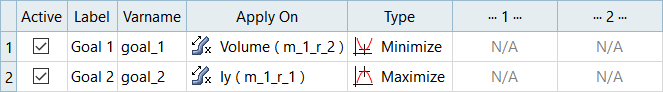
Figure 7. -
Click the More tab and define the following
settings:
- Set Points per Iteration to 4.
- Set Use Inclusion Matrix to Without Initial.
GRSM performs a global search, therefore the initial values of the variables are not important and do not have to be used within the optimization.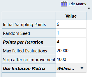
Figure 8. -
Import run data from the DOE using an Inclusion Matrix.
-
Click from the top, right corner of the work area.
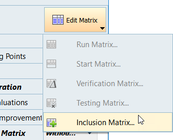
Figure 9.
-
Click from the top, right corner of the work area.
-
Observe the non-dominated front of designs.
These points represent the trade-off between the objective of minimizing volume and maximizing the y-axis moment of inertia. In the plot, it is evident that as the moment of inertia increases, the volume increases as well. This curve represents the trade-off of the best available designs given the competing objective requirements.
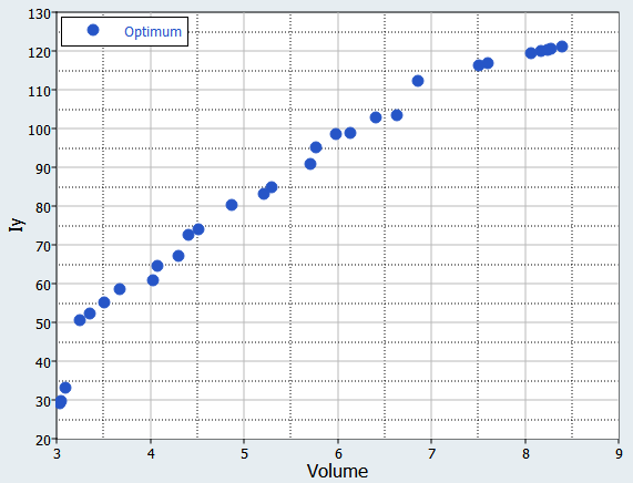
Figure 10. -
Click the Scatter tab to plot the objectives along the
same axes shown in the Optima plot.
This scatter plot shows all of the runs from the optimization. When comparing the scatter and optima plots, note that the optima plot contains only a subset of runs which are non-dominated. A dominated design is a design for which both objectives could be improved. A non-dominated design is one in which one objective may only be improved at the expense of another.
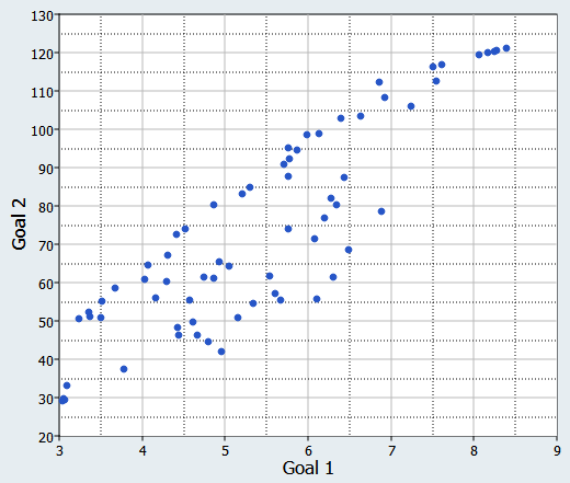
Figure 11.