This tutorial demonstrates how to carry nonlinear analysis for Axi-symmetric ball
joint for pull load of 10,000N using OptiStruct.
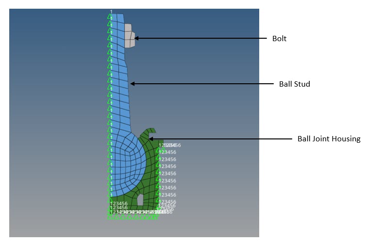
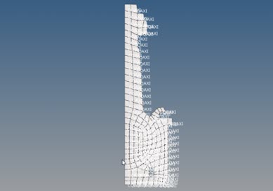
Figure 1 illustrates the structural model used for this
tutorial: Simplified model of Ball joint consisting of ball stud, ball joint housing
and a bolt. It is represented as 2D axisymmetric model. Figure 1. Model and Loading Description
Analysis with a portion of the full model with axi-symmetry boundary conditions. The
following exercises are included:
Set up the Ball Joint 2D axi symmetric analysis in HyperMesh
Submit the job in OptiStruct
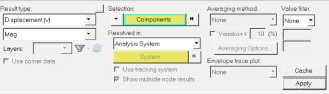
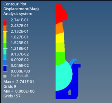
View results in HyperView
Launch HyperMesh and Set the OptiStruct User Profile
Launch HyperMesh.
The User Profile dialog opens.
Select OptiStruct and click
OK.
This loads the user profile. It includes the appropriate template, macro
menu, and import reader, paring down the functionality of HyperMesh to what is relevant for generating models for
OptiStruct.
Open the Model
Click File > Open > Model.
Select the Ball_Joint_2D_Axisymmetry.hm file you saved to
your working directory from the optistruct.zip file. Refer
to Access the Model Files.
Click Open.
The Ball_Joint_2D_Axisymmetry.hm database is loaded
into the current HyperMesh session, replacing any
existing data.
Set Up the Model
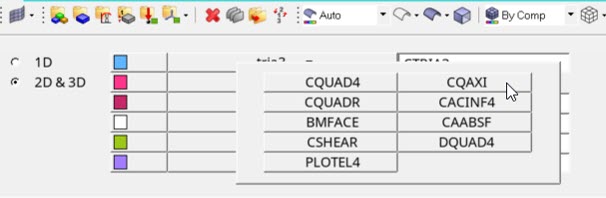
Mesh the Model with CQAXI Elements
The meshed 2D part has CQUAD4 elements and for axisymmetric model
CQAXI elements are used.
Select 2D panel > Element Types.
Activate the 2D&3D panel.
Click CQUAD4, select CQAXI.
Figure 2. Change Element Type
Click elements > displayed.
All the elements displayed are selected.
Click update and return.
From the 2D&3D panel, select elements > displayed.
Click review and return.
Element type is verified. Figure 3. CQAXI Element Type
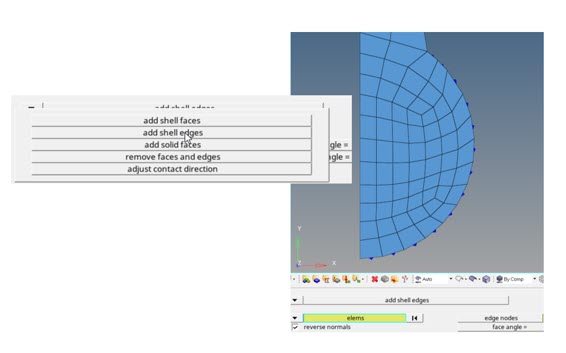
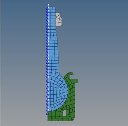
Create Set Segments
This step creates the main surface for the ball stud.
In the Model Browser, right-click and select Create > Set Segment from the context menu.
For Name, enter main.
In the Entity Editor, click on the elements, and select add shell edges > free edges and select the edge of the ball stud where it is in contact with
the housing.
Figure 4. Selection of 2D Elements for Contacts
Deselect the elements which are not in contact with the housing, select
reverse normal and click
add.
The main surface is now created.
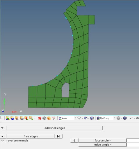
In the Model Browser, right-click and select Create > Set Segment from the context menu.
For Name, enter secondary.
Figure 5. Secondary Contact Elements for Housing
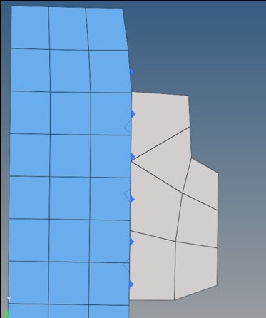
In the Model Browser, right-click and select Create > Set Segment from the context menu.
For Name, enter Main_ball_Stud.
Select the elements of the ball stud which are in contact with the bolt using
shell edges.
Similarly create a contact surface for bolt and rename it to
Secondary_bolt.
Figure 6. Main and Secondary Contact Elements for Ball Stud and
Bolt
Tip: To deselect elements, toggle from free edges to elements and
deselect elements which are not in contact using the Shift and left mouse button.
The contact surfaces for contact between ball stud and bolt is
accomplished.
Create the Contacts
First, you will create the contact between ball stud and housing, then the contact
between bolt and ball stud.
In the Model Browser, right-click and select Create > Contact from the context menu.
For Name, enter CONTACT1.
For Property Option, select static coeffic friction in
the Entity Editor.
For MU1, enter 0.2.
For SSID (Secondary), select Contactsurf from the
drop-down menu and select Secondary surface.
For MSID (Main), select Contactsurf from the drop-down
menu and select main (contact surface).
In the Model Browser, right-click and select Create > Contact from the context menu.
For Name, enter TIE.
For Card Image, select TIE.
For SSID (Secondary), select Secondary_bolt from the
drop-down menu.
For MSID (Main), select Main_ball_stud from the
drop-down menu.
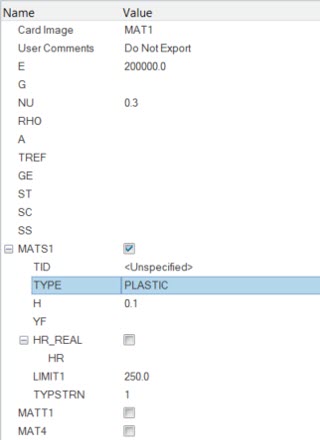
Create the Material
In the Model Browser, right-click and select Create > Material from the context menu.
For Name, enter MAT1.
A new material, MAT1 has beeen
created.
For Card Image, select MAT1.
For NU (Poisson's Ratio), enter 0.3.
Enter the material values next to the corresponding fields.
Figure 7. Material Properties
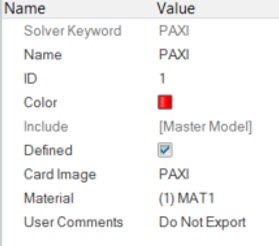
Create the Properties
In the Model Browser, right-click and select Create > Property from the context menu.
For Name, enter PAXI.
For Card Image, select PAXI.
For Material, select MAT1.
Figure 8. Element Property
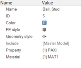
In the Property tab, click on the component ball_stud,
click property and select
PAXI.
In the Property tab, click on the component ball, click
property and select
PAXI.
In the Property tab, click on the component housing,
click property and select
PAXI.
Figure 9. Assign Property to Components
Apply Loads and Boundary Conditions
Create SPCs Load Collector
In the Model Browser, right-click and select Create > Load Collector from the context menu.
A default load collector displays in the Entity Editor.
For Name, enter SPC1.
Click BCs > Create > Constraints to open the Constraints panel.
Select the edge of ball stud edges of 2D Axisymmetric and for only dof-1
(Translational X is fixed), enter 0.
Click Create.
Figure 10. Constraints for Ball Stud
In the Model Browser, right-click and select Create > Load Collector from the context menu.
For Name, enter SPC2.
Click BCs > Create > Constraints to open the Constraints panel.
Select free edges of housing, as shown in Figure 11 and select all dof
1, 2,
3, 4, 5,
6 and enter a value of
0.
All degrees of freedom are fixed.
Click return.
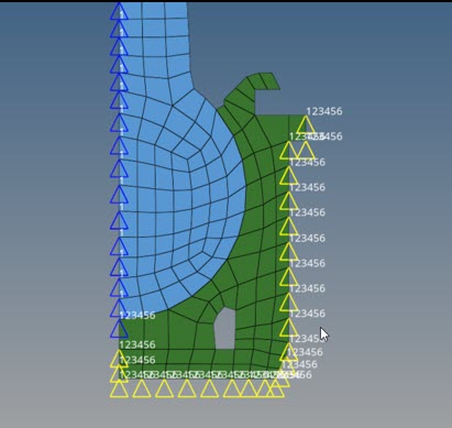
Figure 11. Constraints for Housing
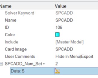
In the Model Browser, right-click and select Create > Load Collector from the context menu.
For Name, enter SPCADD.
For Card Image, select SPCADD.
For SPCADD_NUM_SET, enter 2.
In data set, select SPC1 and
SPC2.
Figure 12. SPCADD
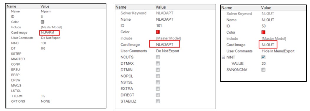
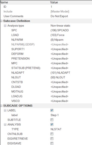
Similarly, create load new load collectors and enter the names as
NLPARM, NLADAPT and
NLOUT.
For Card Images, select the values shown below.
Figure 13. NLPARM, NLADAPT and NLOUT
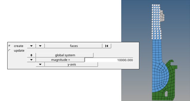
Create Force Load Collector
This step will outline how to apply the force.
In the Model Browser, right-click and select Create > Load Collector from the context menu.
For Name, enter Force.
Click BCs > Create > Force to open the Force panel.
 (Contour).
 from the
panels window.
from the
panels window.