OS-T: 1325 Random Response Analysis of a Flat Plate
This tutorial demonstrates how to set up the random response analysis for the existing frequency response analysis model. The setup for frequency response analysis is that the flat plate has two loading conditions that will be subjected to a frequency-varying load excitation using the direct method.
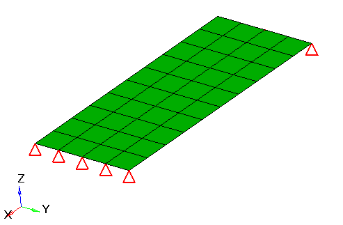
Figure 1.
The frequency analysis setup is already made for this model where the one end of plate is clamped and the loading is applied on the other end (two different sources of the loading, thus two subcases). The loading frequency is defined by the FREQ1 card; from 20 to 1000 Hz with an interval of 20. The same loading frequency is applied on both the subcases.
Launch HyperMesh and Set the OptiStruct User Profile
Open the Model
Set Up the Model
Create Load Collectors
-
Create the tabrnd1 load collector.
-
For data x:, click
 .
.
-
In the TABRND1_NUM= dialog, input the parameters
as shown in Figure 2 and click Close.
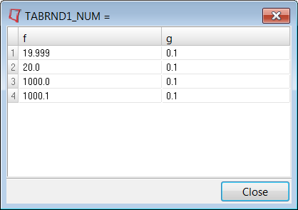
Figure 2.
-
For data x:, click
-
Create the randps load collector.
-
For Data: SID, click .
-
In the NUMBER_OF_RANDPS= dialog, input the
parameters as shown in Figure 3 and click Close.
The TABRND1 load collector is selected for the TID(i) column entries.
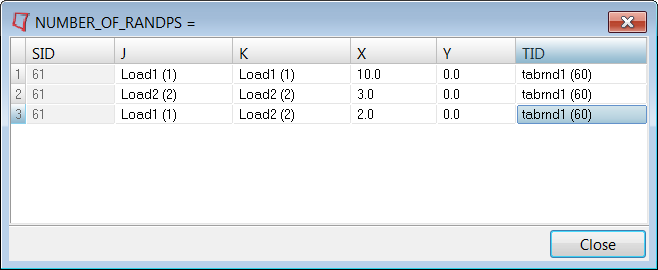
Figure 3.
-
For Data: SID, click
Add Control Cards and Output Requests
Submit the Job
-
From the Analysis page, click the OptiStruct
panel.
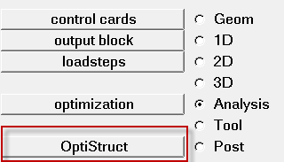
Figure 4. Accessing the OptiStruct Panel
- direct_psd.html
- HTML report of the analysis, providing a summary of the problem formulation and the analysis results.
- direct_psd.out
- OptiStruct output file containing specific information on the file setup, the setup of your optimization problem, estimates for the amount of RAM and disk space required for the run, information for each of the optimization iterations, and compute time information. Review this file for warnings and errors.
- direct_psd.h3d
- HyperView binary results file.
- direct_psd.res
- HyperMesh binary results file.
- direct_psd.stat
- Summary, providing CPU information for each step during analysis process.
- direct_psd.peak
- ASCII result file, containing RMS and peak values of PSD.
- direct_psd.rand
- ASCII result file, containing PSD results.
- direct_psd.mvw
- HyperView script file. This file will automatically create the plot of PSD over the frequency for the results contained in .rand file.
- direct_psd.op2
- Binary file containing RMS and PSD results.
View the Results
This step describes how to post-process the RMS and PSD results in HyperView.
-
Select result type PSD STRESS (t), vonMises, and click
Apply.
The PSD vonMises stress contour at frequency 20.0 Hz are displayed as below:
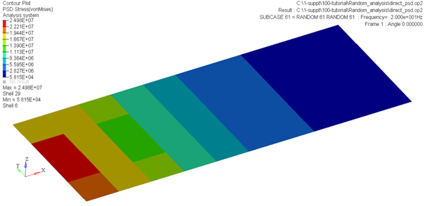
Figure 5. -
Click Open.
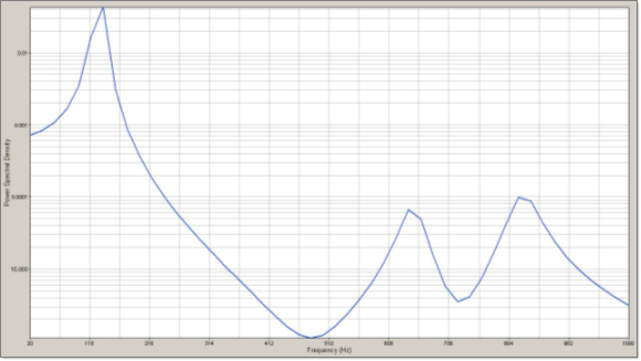
Figure 6.