Direct Matrix Input (Superelements)

The Direct Matrix Input (Superelements) section provides an overview of the following:

Finite Element Analysis (Superelements)

Depending on the analysis type, system equations using these matrices are solved to simulate the structure's behavior. This is referred to as Direct Matrix Input or Superelements.

In the course of a finite element solution, matrix representations of a structure's stiffness, mass, damping, and loading are generated. The matrices are based on the information provided in the Bulk Data section of the input file. For ease of use, this section utilizes Superelements to represent such data.

In a linear static analysis, for example, a system of linear equations is solved. Here K u = f is solved.

Where,
K
Stiffness matrix
f
Loading vector
u
Vector of the unknown displacements
The time taken for these matrix solutions is generally proportional to the square of the number of degrees-of-freedom of the structure. The solution speed can be improved by representing sections of the structure (superelement assemblies) with a smaller subset of degrees of freedom of those sections (boundary degrees of freedom of the superelement assemblies) and a representative set of reduced matrices. In an optimization run, for example, the solution speed can be improved dramatically by removing the non-design portion of the structure and retaining only the design portion of the model.


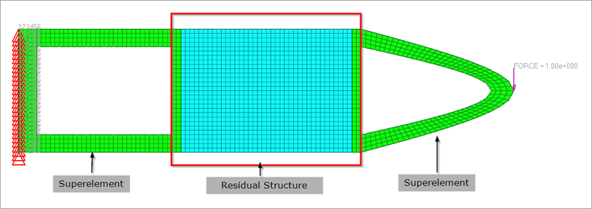
Figure 1. Selecting the Superelements and the Residual Structure

Solving models using superelements is different from the way you run other models in OptiStruct. Therefore, it is beneficial to initially understand a couple of basic terms typically utilized in these solutions.

Direct Matrix Input/Superelement

A superelement is a reduced representation of the behavior and performance of a structure or a part of a structure.

DMIG is the acronym for Direct Matrix Input at Grid points. This matrix is defined by a single header entry and one or more column entries. The DMIG Bulk Data Entry can be used to directly define matrices to be included in the model (such as stiffness and mass matrices). DMIG entries can be selected in the case control section using K2GG, M2GG, B2GG entries and so on for inclusion in the model.

Residual Structure

The part of the full model that remains after the superelement has been created is the Residual structure (or simply, Residual).

The reduced loading, mass, stiffness, and damping matrices can be generated using multiple methods illustrated in subsequent sections. Nevertheless, the basic process involved in using superelements to solve a model can be explained as follows.

Superelement Generation Run

The full-model is carefully examined to determine the sections or parts that can be reduced out as superelements. The boundaries between the superelements and the residual structure are identified using connection/interface points (ASET/BNDFIX/BNDFREE and so on). A variety of factors are involved in the decision to make certain sections of the model into superelements, like computations speedup, sparsity or density of the reduced matrices, type of superelement reduction method, and the type of solution (for example, static versus dynamic). Considerable speedup and ability to perform repeated runs of the model may be possible if the superelement generation run is setup with engineering insight and knowledge. After the identification of interface points, the rest of the structure (residual) is now deleted from the full model. Depending on the superelement creation method selected, the corresponding entries are added (CMSMETH, CDSMETH, and so on). This model is now run in OptiStruct to generate the superelement.

There are three methods available in OptiStruct to generate superelements:
  1. Static Condensation (PARAM, EXTOUT or CMSMETH (GUYAN)) reduces the linear matrix equation to the interface degrees of freedom of the substructure through algebraic substitution. In addition, the load vectors are reduced to the interface degrees of freedom. This includes the load vectors from point and pressure loads as well as distributed loads due to acceleration (GRAV and RLOAD).
    There are two ways to perform static condensation in OptiStruct.
    • Define ASET and PARAM,EXTOUT.
    • Use CMSMETH Bulk Data Entry (with METHOD field set to GUYAN) and CMSMETH Subcase Information Entry.

    Applied loads in the model can be reduced using the USETYPE field on the LOADSET continuation line of the CMSMETH Bulk Data Entry. The USETYPE field can be set to REDLOAD/RESVEC/BOTH.

    For static condensation, only ASET entries are allowed.
    Note: This method is accurate for the stiffness matrix and approximate for the mass matrix.
  2. Dynamic Reduction reduces a finite element model of an elastic body to the interface degrees of freedom and a set of normal modes. The reduced matrices will be generated based on the static modes as well as modes from normal modes analysis.

    The CMSMETH Bulk Data and Subcase Information Entries are used to specify the input for Dynamic Reduction. Supported METHOD types for dynamic reduction is CBN (Craig-Bampton Nodal method) and GM (General method). With GM method, the resulting matrices are always diagonal and they are not physically attached to interface dofs. Therefore, MPC will be generated in residual run to connect the matrices to interface dofs. CBN using CSET also produces the diagonal matrices and this is equivalent to GM with CSET.

    GM with CSET or CBN with CSET could be useful in order to understand the contribution of CMS modes with PFMODE entry.

    Applied loads in the model can be reduced using the USETYPE field on the LOADSET continuation line of the CMSMETH Bulk Data Entry. The USETYPE field can be set to REDLOAD/RESVEC/BOTH. Only static loads can be reduced and it is not supported for METHOD=GM.
    Note: The CBN and GM methods are the preferred method for dynamic analysis as they captures the mass matrix accurately.
  3. Component Dynamic Analysis (CDSMETH) Superelement Generation is efficient for models wherein the residual run is repeated several times. The superelement generation time may be longer than Component Mode Synthesis but the residual run is faster. CDSMETH requires METHOD, FREQi and CSET/CSET1/BNDFRE1,BNDFREE in the generation run. Only Direct Frequency Response Analysis is supported for the Residual run.

Saving Superelements

The reduced matrices can be saved in multiple file formats: .h3d, .pch, .dmg, .op2, and .op4
  • PARAM,EXTOUT,DMIGPCH can be used to output superelements in the .pch format.
  • PARAM,EXTOUT,DMIGBIN can be used to output superelements in the .dmg format.
  • PARAM,EXTOUT,DMIGOP2 can be used to output superelements in the .op2 format.
  • PARAM,EXTOUT,DMIGOP4 can be used to output superelements in the .op4 format.
  • Superelements in .h3d format are always output if CMSMETH entries (Bulk Data and Subcase Information) are present, unless OUTPUT,H3D,NO is set.
    Table 1. Description and Usage Guidelines for Superelements
    Condensation Type Bulk Data Description and Usage Guidelines
    Static Reduction CMSMETH with METHOD=GUYAN Should be used only for static analysis. Not recommended for dynamic analysis as the mass matrices in static reduction are approximated.
    PARAM,EXTOUT
    Dynamic Reduction CMSMETH with METHOD=CBN This is recommended for Dynamic Analysis. Both fixed and free boundary can be used in this method. However, the final reduced mass and stiffness matrices can have off-diagonal terms if fixed boundary is used in the dynamic reduction.
    CMSMETH with METHOD=GM The resulting matrices are always diagonal and they are not physically attached to interface degrees of freedom. Therefore, MPC will be generated in the residual run to connect the matrices to the interface degrees of freedom. Recommended for diagnostic runs with the PFMODE Bulk Data Entry to understand the contribution of modes.

    PARAM,EXTOUT,DMIGOP4 is not applicable for the GM method.

    Component Dynamic Analysis CDSMETH The residual job runs much faster than Component Mode Synthesis because the number of active degree of freedom in the residual run does not depend on the number of modes. This method is efficient for models wherein the residual run is repeated several times.
    Note: The residual run is only supported for direct dynamic analysis. Therefore, the number of degrees of freedom in the residual run should be low (only the connecting elements are recommended).

Residual Run

The superelement created by the generation run is utilized in the residual run. The reduced mass, stiffness, and damping matrices, depending on the type of run, are included with the residual structure. The results are obtained at the requested residual structure grids, elements, other attributes, and at the interface points. To request results in the interior of the superelement, both MODEL entry and the corresponding I/O Options Entry should be specified in the generation run. For additional information, refer to Output.

Superelement Inclusion

For .pch and .dmg files, the name of each matrix should be specified (for example, K2GG for stiffness) in the residual run otherwise, the reduced matrices will not be used. Including the matrices with INCLUDE entries is not sufficient.


Figure 2.
Superelements in H3D format are included via ASSIGN,H3DDMIG in the residual run. For H3D superelements included via H3DDMIG, if the name of matrices are not specified, then all the reduced matrices in H3D file will be utilized. If you specify the name of particular matrices, only such matrices will be used.


Figure 3.

Superelements in OP4 format are included via ASSIGN,OP4DMIG in the residual run. For OP4 superelements included via OP4DMIG, if the name of matrices are not specified, then all the reduced matrices in OP4 file will be utilized. If you specify the name of particular matrices, only such matrices will be used.

Currently, inclusion of .op2 superelements is not supported.

Exterior Point Conversion

The SEINTPNT Subcase Information Entry can be used for residual runs with H3D superelements to convert interior points (dof) of the superelement into exterior points. After this conversion, these degrees of freedom are part of the analysis/optimization degrees of freedom and can be utilized as connection points, loading degrees of freedom, and response degrees of freedom during optimization.

Modify the Superelement

You can modify the superelement in the residual run using the DMIGMOD Bulk Data Entry. This is applicable only to superelements in H3D format.

Damping

Damping is handled differently depending on the type of reduction and the associated attributes of the model. In some cases damping is reduced out in the DMIG generation run. The following sections describe how damping is handled based on the reduction type.

Damping in Static and Dynamic Reduction

Structural damping can be reduced out, by default, if it is defined as GE on material entries (MATi, and so on) or GE on PBUSH, PELAS entries. For global structural damping via PARAM,G an additional parameter PARAM,CMSGDMP,YES should be specified to reduce global damping via PARAM,G.

The SDAMP entry will not be reduced out. If they are applied in the residual run, damping will be applied to the whole model (residual structure as well as the superelement). If SDAMP is required to be applied in each superelement in residual run, this is possible with HYBDAMP option on DMIGMOD Bulk Data Entry.
Table 2. Handling Damping in Static and Dynamic Reduction
Damping Type Reduced out in Generation Run? Comments
Viscous Damping CVISC, CDAMPi, CBUSH (via B on PBUSH) Yes Reduced matrices name would be BA##, where ## is AX by default (can be changed with DMIGNAME).
Modal Viscous Damping via SDAMPING No If SDAMP Subcase Information Entry is specified in residual run, it will be applied to the whole model.

If SDAMP needs to be applied in DMIG in residual run, HYBDAMP option on DMIGMOD can be used.

Rayleigh Damping (via PARAM,ALPHA1 and PARAM,ALPHA2) No (by default)

Yes (if PARAM,CMSGDAMP,YES is specified)

No
If PARAM,ALPHA1/2 is used in residual run, it will be applied to the whole model.
Yes
Damping is reduced out in the generation run. In the residual run, if PARAM,ALPHA1/2 is specified, damping is also applied to the residual structure.
Structural Damping GE on MATi, PBUSH with GE, PELAS with GE Yes Reduced matrices would be named K42## where ## is AX by default (can be changed with DMIGNAME).
PARAM,G No (by default)

Yes (if PARAM,CMSGDAMP,YES is specified)

No
If PARAM,G is used in residual run, it will be applied to the whole model.
Yes
Damping is reduced out in the generation run. In the residual run, if PARAM,G is specified, damping is also applied to the residual structure.

Damping in Component Dynamic Synthesis

Unlike Static Reduction and Dynamic Reduction, any damping in the model (Viscous damping elements, SDAMP, structural damping and so on) will be included in reduced matrices for Component Dynamic Synthesis (CDSMETH).

Mass

PARAM, WTMASS cannot be applied to superelements (.h3d or .pch) that are read into the model. If the unit of mass is incorrect on the MAT# entries and PARAM, WTMASS is required to update the structural mass matrix; then this should be done in the creation run.

Output

Superelements are one of the tools used to reduce model complexity, runtime, and allow confidentiality during model sharing with different teams or companies. As a consequence, by default, output after the residual run is available only for the residual structure.

If output for some sections of the superelements is required, then they can be requested using the MODEL entry and the corresponding output entry. The output will be generated for an intersection of the sets of entities referenced by the MODEL entry and the corresponding output entry.

Example

The following image illustrates the Displacement results of the Residual Structure (only) after the end of the residual run. The output data specified in the input decks is:


Figure 4. Generation Run


Figure 5. Residual Run

direct_matrix_displacement_results
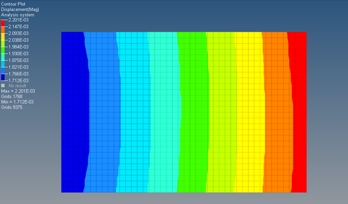
Figure 6. Displacement Results of the Residual Structure (only)
The following image illustrates the Displacement results of the Residual Structure and a set of grid points in the superelement after the end of the residual run. The generation run consists of MODEL data referencing element 10722 (SET 15) and the DISPLACEMENT entry references the grid points associated with element 10722 and some other grid points. You can see how only the results for the intersection of sets referenced by MODEL and the DISPLACEMENT entry is generated. The output data specified in the input decks is:


Figure 7. Generation Run

direct_matrix_resid_run_10722
Figure 8. Residual Run

direct_matrix_displacement_results_10722
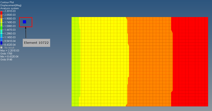
Figure 9. Displacement Results of Residual Structure and Element 10722 in the Superelement

Calculation of derived results (stress, and so on) for interior entities of superelements may be computationally intensive since the corresponding required data is calculated and stored during the generation run. Therefore, it is recommended to only request results for interior sections of the superelement that are critical for the current analysis.

Theory

The following information is common to all superelement generation methods and details the initial partitioning step involved in generating the reduced matrices.

Static Condensation/Reduction is one exception, wherein, the eigenvalue problem shown in this section is not solved.

For the purpose of deriving the reduced matrices, the displacement vector u may be partitioned into displacements of inner, u o and outer, u α interface/attachment degrees of freedom.(1) u=[ u o u a ] MathType@MTEF@5@5@+= feaagKart1ev2aaatCvAUfeBSjuyZL2yd9gzLbvyNv2CaerbuLwBLn hiov2DGi1BTfMBaeXatLxBI9gBaerbd9wDYLwzYbItLDharqqtubsr 4rNCHbGeaGqiVu0Je9sqqrpepC0xbbL8F4rqqrFfpeea0xe9Lq=Jc9 vqaqpepm0xbba9pwe9Q8fs0=yqaqpepae9pg0FirpepeKkFr0xfr=x fr=xb9adbaqaaeGaciGaaiaabeqaamaabaabaaGcbaGaaCyDaiabg2 da9maadmaabaqbaeqabiqaaaqaaiaahwhadaWgaaWcbaGaam4Baaqa baaakeaacaWH1bWaaSbaaSqaaiaadggaaeqaaaaaaOGaay5waiaaw2 faaaaa@3E3B@

Here, the subscript o denotes the inner degrees of freedom, and the α denotes the interface degrees of freedom (for example, ASET entry).

The static equilibrium is given as:(2) [ K oo K oa K oa T K aa ][ u o u a ]=[ f o f a ] MathType@MTEF@5@5@+= feaagKart1ev2aqatCvAUfeBSjuyZL2yd9gzLbvyNv2CaerbuLwBLn hiov2DGi1BTfMBaeXatLxBI9gBaerbd9wDYLwzYbItLDharqqtubsr 4rNCHbGeaGqiVu0Je9sqqrpepC0xbbL8F4rqqrFfpeea0xe9Lq=Jc9 vqaqpepm0xbba9pwe9Q8fs0=yqaqpepae9pg0FirpepeKkFr0xfr=x fr=xb9adbaqaaeGaciGaaiaabeqaamaabaabaaGcbaWaamWaaeaafa qabeGacaaabaGaaC4samaaBaaaleaacaWGVbGaam4Baaqabaaakeaa caWHlbWaaSbaaSqaaiaad+gacaWGHbaabeaaaOqaaiaahUeadaqhaa WcbaGaam4BaiaadggaaeaacaWGubaaaaGcbaGaaC4samaaBaaaleaa caWGHbGaamyyaaqabaaaaaGccaGLBbGaayzxaaWaamWaaeaafaqabe GabaaabaGaaCyDamaaBaaaleaacaWGVbaabeaaaOqaaiaahwhadaWg aaWcbaGaamyyaaqabaaaaaGccaGLBbGaayzxaaGaeyypa0ZaamWaae aafaqabeGabaaabaGaaCOzamaaBaaaleaacaWGVbaabeaaaOqaaiaa hAgadaWgaaWcbaGaamyyaaqabaaaaaGccaGLBbGaayzxaaaaaa@51CD@

Where, K is the stiffness matrix and f is the force vector with the corresponding subscripts depicting the partitioning based on the inner/interface degrees of freedom.

For CBN and GM methods, an eigenvalue analysis is also performed to generate the eigenmodes.

The eigenvalue problem for a normal modes analysis of the body using a diagonal mass matrix, M is:(3) [ [ K oo K oa K oa T K aa ]λ[ M oo 0 0 M aa ] ][ A o A a ]=[ 0 0 ] MathType@MTEF@5@5@+= feaagKart1ev2aqatCvAUfeBSjuyZL2yd9gzLbvyNv2CaerbuLwBLn hiov2DGi1BTfMBaeXatLxBI9gBaerbd9wDYLwzYbItLDharqqtubsr 4rNCHbGeaGqiVu0Je9sqqrpepC0xbbL8F4rqqrFfpeea0xe9Lq=Jc9 vqaqpepm0xbba9pwe9Q8fs0=yqaqpepae9pg0FirpepeKkFr0xfr=x fr=xb9adbaqaaeGaciGaaiaabeqaamaabaabaaGcbaWaamWaaeaada WadaqaauaabeqaciaaaeaacaWHlbWaaSbaaSqaaiaad+gacaWGVbaa beaaaOqaaiaahUeadaWgaaWcbaGaam4BaiaadggaaeqaaaGcbaGaaC 4samaaDaaaleaacaWGVbGaamyyaaqaaiaadsfaaaaakeaacaWHlbWa aSbaaSqaaiaadggacaWGHbaabeaaaaaakiaawUfacaGLDbaacqGHsi slcqaH7oaBdaWadaqaauaabeqaciaaaeaacaWHnbWaaSbaaSqaaiaa d+gacaWGVbaabeaaaOqaaiaaicdaaeaacaaIWaaabaGaaCytamaaBa aaleaacaWGHbGaamyyaaqabaaaaaGccaGLBbGaayzxaaaacaGLBbGa ayzxaaWaamWaaeaafaqabeGabaaabaGaaCyqamaaBaaaleaacaWGVb aabeaaaOqaaiaahgeadaWgaaWcbaGaamyyaaqabaaaaaGccaGLBbGa ayzxaaGaeyypa0ZaamWaaeaafaqabeGabaaabaGaaGimaaqaaiaaic daaaaacaGLBbGaayzxaaaaaa@5C8A@

Where, A are the partitioned eigenvectors of the system. Only eigenvectors pertaining to the non-attachment degrees of freedom, A o , are used in the subsequent generation of the combined modal matrix (see Craig Bampton Nodal Method (CBN) and General Method (GM)).

Static Condensation (PARAM, EXTOUT or CMSMETH (GUYAN))

The first line of Equation 2 reads as:(4) K oo u o + K oa u a = f o MathType@MTEF@5@5@+= feaagKart1ev2aqatCvAUfeBSjuyZL2yd9gzLbvyNv2CaerbuLwBLn hiov2DGi1BTfMBaeXatLxBI9gBaerbd9wDYLwzYbItLDharqqtubsr 4rNCHbGeaGqiVu0Je9sqqrpepC0xbbL8F4rqqrFfpeea0xe9Lq=Jc9 vqaqpepm0xbba9pwe9Q8fs0=yqaqpepae9pg0FirpepeKkFr0xfr=x fr=xb9adbaqaaeGaciGaaiaabeqaamaabaabaaGcbaGaaC4samaaBa aaleaacaWGVbGaam4BaaqabaGccaWH1bWaaSbaaSqaaiaad+gaaeqa aOGaey4kaSIaaC4samaaBaaaleaacaWGVbGaamyyaaqabaGccaWH1b WaaSbaaSqaaiaadggaaeqaaOGaeyypa0JaaCOzamaaBaaaleaacaWG Vbaabeaaaaa@4406@
The displacements of the inner degrees of freedom, therefore are:(5) u o = K oo 1 [ f o K oa u a ] MathType@MTEF@5@5@+= feaagKart1ev2aqatCvAUfeBSjuyZL2yd9gzLbvyNv2CaerbuLwBLn hiov2DGi1BTfMBaeXatLxBI9gBaerbd9wDYLwzYbItLDharqqtubsr 4rNCHbGeaGqiVu0Je9sqqrpepC0xbbL8F4rqqrFfpeea0xe9Lq=Jc9 vqaqpepm0xbba9pwe9Q8fs0=yqaqpepae9pg0FirpepeKkFr0xfr=x fr=xb9adbaqaaeGaciGaaiaabeqaamaabaabaaGcbaGaaCyDamaaBa aaleaacaWGVbaabeaakiabg2da9iaahUeadaqhaaWcbaGaam4Baiaa d+gaaeaacqGHsislcaaIXaaaaOWaamWaaeaacaWHMbWaaSbaaSqaai aad+gaaeqaaOGaeyOeI0IaaC4samaaBaaaleaacaWGVbGaamyyaaqa baGccaWH1bWaaSbaaSqaaiaadggaaeqaaaGccaGLBbGaayzxaaaaaa@47B6@

u a MathType@MTEF@5@5@+= feaagKart1ev2aqatCvAUfeBSjuyZL2yd9gzLbvyNv2CaerbuLwBLn hiov2DGi1BTfMBaeXatLxBI9gBaerbd9wDYLwzYbItLDharqqtubsr 4rNCHbGeaGqiVu0Je9sqqrpepC0xbbL8F4rqqrFfpeea0xe9Lq=Jc9 vqaqpepm0xbba9pwe9Q8fs0=yqaqpepae9pg0FirpepeKkFr0xfr=x fr=xb9adbaqaaeGaciGaaiaabeqaamaabaabaaGcbaGaaCyDamaaBa aaleaacaWGHbaabeaaaaa@3807@ solving for u o

Also from Equation 2:(6) K ao u o + K aa u a = f a MathType@MTEF@5@5@+= feaagKart1ev2aqatCvAUfeBSjuyZL2yd9gzLbvyNv2CaerbuLwBLn hiov2DGi1BTfMBaeXatLxBI9gBaerbd9wDYLwzYbItLDharqqtubsr 4rNCHbGeaGqiVu0Je9sqqrpepC0xbbL8F4rqqrFfpeea0xe9Lq=Jc9 vqaqpepm0xbba9pwe9Q8fs0=yqaqpepae9pg0FirpepeKkFr0xfr=x fr=xb9adbaqaaeGaciGaaiaabeqaamaabaabaaGcbaGaaC4samaaBa aaleaacaWGHbGaam4BaaqabaGccaWH1bWaaSbaaSqaaiaad+gaaeqa aOGaey4kaSIaaC4samaaBaaaleaacaWGHbGaamyyaaqabaGccaWH1b WaaSbaaSqaaiaadggaaeqaaOGaeyypa0JaaCOzamaaBaaaleaacaWG Hbaabeaaaaa@43DC@
Substituting Equation 5 into this:(7) K ao K oo 1 [ f o K oa u a ]+ K aa u a = f a MathType@MTEF@5@5@+= feaagKart1ev2aqatCvAUfeBSjuyZL2yd9gzLbvyNv2CaerbuLwBLn hiov2DGi1BTfMBaeXatLxBI9gBaerbd9wDYLwzYbItLDharqqtubsr 4rNCHbGeaGqiVu0Je9sqqrpepC0xbbL8F4rqqrFfpeea0xe9Lq=Jc9 vqaqpepm0xbba9pwe9Q8fs0=yqaqpepae9pg0FirpepeKkFr0xfr=x fr=xb9adbaqaaeGaciGaaiaabeqaamaabaabaaGcbaGaaC4samaaBa aaleaacaWGHbGaam4BaaqabaGccaWHlbWaa0baaSqaaiaad+gacaWG VbaabaGaeyOeI0IaaGymaaaakmaadmaabaGaaCOzamaaBaaaleaaca WGVbaabeaakiabgkHiTiaahUeadaWgaaWcbaGaam4Baiaadggaaeqa aOGaaCyDamaaBaaaleaacaWGHbaabeaaaOGaay5waiaaw2faaiabgU caRiaahUeadaWgaaWcbaGaamyyaiaadggaaeqaaOGaaCyDamaaBaaa leaacaWGHbaabeaakiabg2da9iaahAgadaWgaaWcbaGaamyyaaqaba aaaa@5045@
or(8) [ K aa K ao K oo 1 K oa ] u a = f a K ao K oo 1 f o MathType@MTEF@5@5@+= feaagKart1ev2aqatCvAUfeBSjuyZL2yd9gzLbvyNv2CaerbuLwBLn hiov2DGi1BTfMBaeXatLxBI9gBaerbd9wDYLwzYbItLDharqqtubsr 4rNCHbGeaGqiVu0Je9sqqrpepC0xbbL8F4rqqrFfpeea0xe9Lq=Jc9 vqaqpepm0xbba9pwe9Q8fs0=yqaqpepae9pg0FirpepeKkFr0xfr=x fr=xb9adbaqaaeGaciGaaiaabeqaamaabaabaaGcbaWaamWaaeaaca WHlbWaaSbaaSqaaiaadggacaWGHbaabeaakiabgkHiTiaahUeadaWg aaWcbaGaamyyaiaad+gaaeqaaOGaaC4samaaDaaaleaacaWGVbGaam 4BaaqaaiabgkHiTiaaigdaaaGccaWHlbWaaSbaaSqaaiaad+gacaWG HbaabeaaaOGaay5waiaaw2faaiaahwhadaWgaaWcbaGaamyyaaqaba GccqGH9aqpcaWHMbWaaSbaaSqaaiaadggaaeqaaOGaeyOeI0IaaC4s amaaBaaaleaacaWGHbGaam4BaaqabaGccaWHlbWaa0baaSqaaiaad+ gacaWGVbaabaGaeyOeI0IaaGymaaaakiaahAgadaWgaaWcbaGaam4B aaqabaaaaa@55B5@
This is interpreted as:(9) K reduced u a = f reduced MathType@MTEF@5@5@+= feaagKart1ev2aqatCvAUfeBSjuyZL2yd9gzLbvyNv2CaerbuLwBLn hiov2DGi1BTfMBaeXatLxBI9gBaerbd9wDYLwzYbItLDharqqtubsr 4rNCHbGeaGqiVu0Je9sqqrpepC0xbbL8F4rqqrFfpeea0xe9Lq=Jc9 vqaqpepm0xbba9pwe9Q8fs0=yqaqpepae9pg0FirpepeKkFr0xfr=x fr=xb9adbaqaaeGaciGaaiaabeqaamaabaabaaGcbaGaaC4samaaBa aaleaacaWGYbGaamyzaiaadsgacaWG1bGaam4yaiaadwgacaWGKbaa beaakiaahwhadaWgaaWcbaGaamyyaaqabaGccqGH9aqpcaWHMbWaaS baaSqaaiaadkhacaWGLbGaamizaiaadwhacaWGJbGaamyzaiaadsga aeqaaaaa@483A@
So the reduced stiffness is:(10) K reduced = K aa K ao K oo 1 K oa MathType@MTEF@5@5@+= feaagKart1ev2aqatCvAUfeBSjuyZL2yd9gzLbvyNv2CaerbuLwBLn hiov2DGi1BTfMBaeXatLxBI9gBaerbd9wDYLwzYbItLDharqqtubsr 4rNCHbGeaGqiVu0Je9sqqrpepC0xbbL8F4rqqrFfpeea0xe9Lq=Jc9 vqaqpepm0xbba9pwe9Q8fs0=yqaqpepae9pg0FirpepeKkFr0xfr=x fr=xb9adbaqaaeGaciGaaiaabeqaamaabaabaaGcbaGaaC4samaaBa aaleaacaWGYbGaamyzaiaadsgacaWG1bGaam4yaiaadwgacaWGKbaa beaakiabg2da9iaahUeadaWgaaWcbaGaamyyaiaadggaaeqaaOGaey OeI0IaaC4samaaBaaaleaacaWGHbGaam4BaaqabaGccaWHlbWaa0ba aSqaaiaad+gacaWGVbaabaGaeyOeI0IaaGymaaaakiaahUeadaWgaa WcbaGaam4Baiaadggaaeqaaaaa@4CA2@
And the reduced loading is:(11) f reduced = f a K ao K oo 1 f o MathType@MTEF@5@5@+= feaagKart1ev2aqatCvAUfeBSjuyZL2yd9gzLbvyNv2CaerbuLwBLn hiov2DGi1BTfMBaeXatLxBI9gBaerbd9wDYLwzYbItLDharqqtubsr 4rNCHbGeaGqiVu0Je9sqqrpepC0xbbL8F4rqqrFfpeea0xe9Lq=Jc9 vqaqpepm0xbba9pwe9Q8fs0=yqaqpepae9pg0FirpepeKkFr0xfr=x fr=xb9adbaqaaeGaciGaaiaabeqaamaabaabaaGcbaGaaCOzamaaBa aaleaacaWGYbGaamyzaiaadsgacaWG1bGaam4yaiaadwgacaWGKbaa beaakiabg2da9iaahAgadaWgaaWcbaGaamyyaaqabaGccqGHsislca WHlbWaaSbaaSqaaiaadggacaWGVbaabeaakiaahUeadaqhaaWcbaGa am4Baiaad+gaaeaacqGHsislcaaIXaaaaOGaaCOzamaaBaaaleaaca WGVbaabeaaaaa@4B27@
The reduced matrix can now also be written based on the displacement matrix, S MathType@MTEF@5@5@+= feaagKart1ev2aaatCvAUfeBSjuyZL2yd9gzLbvyNv2CaerbuLwBLn hiov2DGi1BTfMBaeXatLxBI9gBaerbd9wDYLwzYbItLDharqqtubsr 4rNCHbGeaGqiVu0Je9sqqrpepC0xbbL8F4rqqrFfpeea0xe9Lq=Jc9 vqaqpepm0xbba9pwe9Q8fs0=yqaqpepae9pg0FirpepeKkFr0xfr=x fr=xb9adbaqaaeGaciGaaiaabeqaamaabaabaaGcbaGaaC4uaaaa@36D2@ :(12) K reduced = S T KS= K aa K ao K oo 1 K oa MathType@MTEF@5@5@+= feaagKart1ev2aqatCvAUfeBSjuyZL2yd9gzLbvyNv2CaerbuLwBLn hiov2DGi1BTfMBaeXatLxBI9gBaerbd9wDYLwzYbItLDharqqtubsr 4rNCHbGeaGqiVu0Je9sqqrpepC0xbbL8F4rqqrFfpeea0xe9Lq=Jc9 vqaqpepm0xbba9pwe9Q8fs0=yqaqpepae9pg0FirpepeKkFr0xfr=x fr=xb9adbaqaaeGaciGaaiaabeqaamaabaabaaGcbaGaaC4samaaBa aaleaacaWGYbGaamyzaiaadsgacaWG1bGaam4yaiaadwgacaWGKbaa beaakiabg2da9iaahofadaahaaWcbeqaaiaadsfaaaGccaWHlbGaaC 4uaiabg2da9iaahUeadaWgaaWcbaGaamyyaiaadggaaeqaaOGaeyOe I0IaaC4samaaBaaaleaacaWGHbGaam4BaaqabaGccaWHlbWaa0baaS qaaiaad+gacaWGVbaabaGaeyOeI0IaaGymaaaakiaahUeadaWgaaWc baGaam4Baiaadggaaeqaaaaa@5144@
Then, using a similar transformation, you can obtain the reduced mass matrix:(13) M reduced = S T MS= M aa + K ao K oo 1 M oa K oo 1 K oa K ao K oo 1 M oa M ao K oo 1 K oa MathType@MTEF@5@5@+= feaagKart1ev2aqatCvAUfeBSjuyZL2yd9gzLbvyNv2CaerbuLwBLn hiov2DGi1BTfMBaeXatLxBI9gBaerbd9wDYLwzYbItLDharqqtubsr 4rNCHbGeaGqiVu0Je9sqqrpepC0xbbL8F4rqqrFfpeea0xe9Lq=Jc9 vqaqpepm0xbba9pwe9Q8fs0=yqaqpepae9pg0FirpepeKkFr0xfr=x fr=xb9adbaqaaeGaciGaaiaabeqaamaabaabaaGcbaGaaCytamaaBa aaleaacaWGYbGaamyzaiaadsgacaWG1bGaam4yaiaadwgacaWGKbaa beaakiabg2da9iaahofadaahaaWcbeqaaiaadsfaaaGccaWHnbGaaC 4uaiabg2da9iaah2eadaWgaaWcbaGaamyyaiaadggaaeqaaOGaey4k aSIaaC4samaaBaaaleaacaWGHbGaam4BaaqabaGccaWHlbWaa0baaS qaaiaad+gacaWGVbaabaGaeyOeI0IaaGymaaaakiaah2eadaWgaaWc baGaam4BaiaadggaaeqaaOGaaC4samaaDaaaleaacaWGVbGaam4Baa qaaiabgkHiTiaaigdaaaGccaWHlbWaaSbaaSqaaiaad+gacaWGHbaa beaakiabgkHiTiaahUeadaWgaaWcbaGaamyyaiaad+gaaeqaaOGaaC 4samaaDaaaleaacaWGVbGaam4BaaqaaiabgkHiTiaaigdaaaGccaWH nbWaaSbaaSqaaiaad+gacaWGHbaabeaakiabgkHiTiaah2eadaWgaa WcbaGaamyyaiaad+gaaeqaaOGaaC4samaaDaaaleaacaWGVbGaam4B aaqaaiabgkHiTiaaigdaaaGccaWHlbWaaSbaaSqaaiaad+gacaWGHb aabeaaaaa@6F64@

The solution of the reduced linear static problem provides an exact solution, whereas the solution of the reduced eigenvalue problem, K r e d u c e d u a = λ M r e d u c e d u a MathType@MTEF@5@5@+= feaagKart1ev2aqatCvAUfeBSjuyZL2yd9gzLbvyNv2CaerbuLwBLn hiov2DGi1BTfMBaeXatLxBI9gBaerbd9wDYLwzYbItLDharqqtubsr 4rNCHbGeaGqiVu0Je9sqqrpepC0xbbL8F4rqqrFfpeea0xe9Lq=Jc9 vqaqpepm0xbba9pwe9Q8fs0=yqaqpepae9pg0FirpepeKkFr0xfr=x fr=xb9adbaqaaeGaciGaaiaabeqaamaabaabaaGcbaGaaC4samaaBa aaleaacaWGYbGaamyzaiaadsgacaWG1bGaam4yaiaadwgacaWGKbaa beaakiaahwhadaWgaaWcbaGaamyyaaqabaGccqGH9aqpcqaH7oaBca WHnbWaaSbaaSqaaiaadkhacaWGLbGaamizaiaadwhacaWGJbGaamyz aiaadsgaaeqaaOGaaCyDamaaBaaaleaacaWGHbaabeaaaaa@4BEF@ , only provides approximations to the solution of the full eigenvalue problem as only vectors that satisfy the constraint u o = K o o 1 K o a u a MathType@MTEF@5@5@+= feaagKart1ev2aqatCvAUfeBSjuyZL2yd9gzLbvyNv2CaerbuLwBLn hiov2DGi1BTfMBaeXatLxBI9gBaerbd9wDYLwzYbItLDharqqtubsr 4rNCHbGeaGqiVu0Je9sqqrpepC0xbbL8F4rqqrFfpeea0xe9Lq=Jc9 vqaqpepm0xbba9pwe9Q8fs0=yqaqpepae9pg0FirpepeKkFr0xfr=x fr=xb9adbaqaaeGaciGaaiaabeqaamaabaabaaGcbaGaaCyDamaaBa aaleaacaWGVbaabeaakiabg2da9iabgkHiTiaahUeadaqhaaWcbaGa am4Baiaad+gaaeaacqGHsislcaaIXaaaaOGaaC4samaaBaaaleaaca WGVbGaamyyaaqabaGccaWH1bWaaSbaaSqaaiaadggaaeqaaaaa@43A1@ will be included in the solution. This can be explained by illustrating that the displacement matrix, S MathType@MTEF@5@5@+= feaagKart1ev2aaatCvAUfeBSjuyZL2yd9gzLbvyNv2CaerbuLwBLn hiov2DGi1BTfMBaeXatLxBI9gBaerbd9wDYLwzYbItLDharqqtubsr 4rNCHbGeaGqiVu0Je9sqqrpepC0xbbL8F4rqqrFfpeea0xe9Lq=Jc9 vqaqpepm0xbba9pwe9Q8fs0=yqaqpepae9pg0FirpepeKkFr0xfr=x fr=xb9adbaqaaeGaciGaaiaabeqaamaabaabaaGcbaGaaC4uaaaa@36D2@ only consists of static displacement modes (represented by A s MathType@MTEF@5@5@+= feaagKart1ev2aqatCvAUfeBSjuyZL2yd9gzLbvyNv2CaerbuLwBLn hiov2DGi1BTfMBaeXatLxBI9gBaerbd9wDYLwzYbItLDharqqtubsr 4rNCHbGeaGqiVu0Je9sqqrpepC0xbbL8F4rqqrFfpeea0xe9Lq=Jc9 vqaqpepm0xbba9pwe9Q8fs0=yqaqpepae9pg0FirpepeKkFr0xfr=x fr=xb9adbaqaaeGaciGaaiaabeqaamaabaabaaGcbaGaaCyqamaaBa aaleaacaWGZbaabeaaaaa@37E5@ ). The eigenmodes (represented by A ω MathType@MTEF@5@5@+= feaagKart1ev2aqatCvAUfeBSjuyZL2yd9gzLbvyNv2CaerbuLwBLn hiov2DGi1BTfMBaeXatLxBI9gBaerbd9wDYLwzYbItLDharqqtubsr 4rNCHbGeaGqiVu0Je9sqqrpepC0xbbL8F4rqqrFfpeea0xe9Lq=Jc9 vqaqpepm0xbba9pwe9Q8fs0=yqaqpepae9pg0FirpepeKkFr0xfr=x fr=xb9adbaqaaeGaciGaaiaabeqaamaabaabaaGcbaGaaCyqamaaBa aaleaacqaHjpWDaeqaaaaa@38BA@ ) are not calculated in Static Condensation, therefore the reduced mass matrix is approximate.

Compliance Results for Reduced Models

If external forces are applied to the degrees of freedom that are reduced out of the model, then the strain energy or compliance values for the complete model will not match the strain energy or compliance values for the reduced model.

From the previous section, the reduced loading is written as:(14) f reduced = f a K ao K oo 1 f o MathType@MTEF@5@5@+= feaagKart1ev2aqatCvAUfeBSjuyZL2yd9gzLbvyNv2CaerbuLwBLn hiov2DGi1BTfMBaeXatLxBI9gBaerbd9wDYLwzYbItLDharqqtubsr 4rNCHbGeaGqiVu0Je9sqqrpepC0xbbL8F4rqqrFfpeea0xe9Lq=Jc9 vqaqpepm0xbba9pwe9Q8fs0=yqaqpepae9pg0FirpepeKkFr0xfr=x fr=xb9adbaqaaeGaciGaaiaabeqaamaabaabaaGcbaGaaCOzamaaBa aaleaacaWGYbGaamyzaiaadsgacaWG1bGaam4yaiaadwgacaWGKbaa beaakiabg2da9iaahAgadaWgaaWcbaGaamyyaaqabaGccqGHsislca WHlbWaaSbaaSqaaiaadggacaWGVbaabeaakiaahUeadaqhaaWcbaGa am4Baiaad+gaaeaacqGHsislcaaIXaaaaOGaaCOzamaaBaaaleaaca WGVbaabeaaaaa@4B27@
Therefore, strain energy for the reduced model is:(15) 1 2 u a f reduced = 1 2 [ u a f a u a K ao K oo 1 f o ] MathType@MTEF@5@5@+= feaagKart1ev2aqatCvAUfeBSjuyZL2yd9gzLbvyNv2CaerbuLwBLn hiov2DGi1BTfMBaeXatLxBI9gBaerbd9wDYLwzYbItLDharqqtubsr 4rNCHbGeaGqiVu0Je9sqqrpepC0xbbL8F4rqqrFfpeea0xe9Lq=Jc9 vqaqpepm0xbba9pwe9Q8fs0=yqaqpepae9pg0FirpepeKkFr0xfr=x fr=xb9adbaqaaeGaciGaaiaabeqaamaabaabaaGcbaWaaSGaaeaaca aIXaaabaGaaGOmaaaacaWH1bWaaSbaaSqaaiaadggaaeqaaOGaaCOz amaaBaaaleaacaWGYbGaamyzaiaadsgacaWG1bGaam4yaiaadwgaca WGKbaabeaakiabg2da9maaliaabaGaaGymaaqaaiaaikdaaaWaamWa aeaacaWH1bWaaSbaaSqaaiaadggaaeqaaOGaaCOzamaaBaaaleaaca WGHbaabeaakiabgkHiTiaahwhadaWgaaWcbaGaamyyaaqabaGccaWH lbWaaSbaaSqaaiaadggacaWGVbaabeaakiaahUeadaqhaaWcbaGaam 4Baiaad+gaaeaacqGHsislcaaIXaaaaOGaaCOzamaaBaaaleaacaWG VbaabeaaaOGaay5waiaaw2faaaaa@5683@
The strain energy for the complete model is:(16) 1 2 uf= 1 2 [ u a f a + u o f o ]= 1 2 [ u a f a u a K ao K oo 1 f o + f o K oo 1 f o ] MathType@MTEF@5@5@+= feaagKart1ev2aqatCvAUfeBSjuyZL2yd9gzLbvyNv2CaerbuLwBLn hiov2DGi1BTfMBaeXatLxBI9gBaerbd9wDYLwzYbItLDharqqtubsr 4rNCHbGeaGqiVu0Je9sqqrpepC0xbbL8F4rqqrFfpeea0xe9Lq=Jc9 vqaqpepm0xbba9pwe9Q8fs0=yqaqpepae9pg0FirpepeKkFr0xfr=x fr=xb9adbaqaaeGaciGaaiaabeqaamaabaabaaGcbaWaaSGaaeaaca aIXaaabaGaaGOmaaaacaWH1bGaaCOzaiabg2da9maaliaabaGaaGym aaqaaiaaikdaaaWaamWaaeaacaWH1bWaaSbaaSqaaiaadggaaeqaaO GaaCOzamaaBaaaleaacaWGHbaabeaakiabgUcaRiaahwhadaWgaaWc baGaam4BaaqabaGccaWHMbWaaSbaaSqaaiaad+gaaeqaaaGccaGLBb GaayzxaaGaeyypa0ZaaSGaaeaacaaIXaaabaGaaGOmaaaadaWadaqa aiaahwhadaWgaaWcbaGaamyyaaqabaGccaWHMbWaaSbaaSqaaiaadg gaaeqaaOGaeyOeI0IaaCyDamaaBaaaleaacaWGHbaabeaakiaahUea daWgaaWcbaGaamyyaiaad+gaaeqaaOGaaC4samaaDaaaleaacaWGVb Gaam4BaaqaaiabgkHiTiaaigdaaaGccaWHMbWaaSbaaSqaaiaad+ga aeqaaOGaey4kaSIaaCOzamaaBaaaleaacaWGVbaabeaakiaahUeada qhaaWcbaGaam4Baiaad+gaaeaacqGHsislcaaIXaaaaOGaaCOzamaa BaaaleaacaWGVbaabeaaaOGaay5waiaaw2faaaaa@662A@

Comparing the two equations, you can see that the compliance for the reduced model is missing the term, f o K oo 1 f o MathType@MTEF@5@5@+= feaagKart1ev2aaatCvAUfeBSjuyZL2yd9gzLbvyNv2CaerbuLwBLn hiov2DGi1BTfMBaeXatLxBI9gBaerbd9wDYLwzYbItLDharqqtubsr 4rNCHbGeaGqiVu0Je9sqqrpepC0xbbL8F4rqqrFfpeea0xe9Lq=Jc9 vqaqpepm0xbba9pwe9Q8fs0=yqaqpepae9pg0FirpepeKkFr0xfr=x fr=xb9adbaqaaeGaciGaaiaabeqaamaabaabaaGcbaGaaCOzamaaBa aaleaacaWGVbaabeaakiaahUeadaqhaaWcbaGaam4Baiaad+gaaeaa cqGHsislcaaIXaaaaOGaaCOzamaaBaaaleaacaWGVbaabeaaaaa@3EB9@ .

When no external forces are applied to the degrees of freedom that are reduced out of the model, then f o MathType@MTEF@5@5@+= feaagKart1ev2aqatCvAUfeBSjuyZL2yd9gzLbvyNv2CaerbuLwBLn hiov2DGi1BTfMBaeXatLxBI9gBaerbd9wDYLwzYbItLDharqqtubsr 4rNCHbGeaGqiVu0Je9sqqrpepC0xbbL8F4rqqrFfpeea0xe9Lq=Jc9 vqaqpepm0xbba9pwe9Q8fs0=yqaqpepae9pg0FirpepeKkFr0xfr=x fr=xb9adbeqaaeGaciGaaiaabeqaamaabaabaaGcbaGaaeOzamaaBa aaleaacaWGVbaabeaaaaa@3801@ is equal to zero, and the strain energy or compliance values for the reduced model match the complete model.

Dynamic Condensation (CMSMETH (CBN/GM))

Dynamic Condensation consists of both static modes and eigenmodes.

The interface or boundary degrees of freedom that are used in the construction of mode shapes should be representative of the set of force-bearing degrees of freedom in the subsequent analysis. For a finite element analysis, this refers to those nodes that connect to either the residual structure or other super element assemblies.

Supported Bulk Data Entry for interface degrees of freedom are: ASET/ASET1, BSET/BSET1, CSET/CSET1, BNDFIX/BNDFIX1, and BNDFREE/BNDFRE1. These Bulk Data Entries define the interface dofs to be constrained or freed.

The purpose of specifying the interface or boundary degrees of freedom for CMS is mainly to account for the static deformation due to constraint or applied forces acting on the interface degrees of freedom. A large number of eigenmodes is required, if these static modes are omitted. The flexible deformations due to constraint forces, compared to the deformation due to the body inertia forces, are often dominant in most constrained models. The inclusion of all force-bearing degrees of freedom as interface degrees of freedom is therefore an essential step to get accurate results from subsequent analyses.

The METHOD field can be set to CBN or GM on the CMSMETH Bulk Data Entry for activation.

Craig Bampton Nodal Method (CBN)

Normal modes analysis of the fixed-interface system yields the diagonal matrix of eigenvalues, D ω MathType@MTEF@5@5@+= feaagKart1ev2aaatCvAUfeBSjuyZL2yd9gzLbvyNv2CaerbuLwBLn hiov2DGi1BTfMBaeXatLxBI9gBaerbd9wDYLwzYbItLDharqqtubsr 4rNCHbGeaGqiVu0Je9sqqrpepC0xbbL8F4rqqrFfpeea0xe9Lq=Jc9 vqaqpepm0xbba9pwe9Q8fs0=yqaqpepae9pg0FirpepeKkFr0xfr=x fr=xb9adbaqaaeGaciGaaiaabeqaamaabaabaaGcbaGaaCyqamaaBa aaleaacqaHjpWDaeqaaaaa@38B9@ and the matrix of eigenmodes, A ω MathType@MTEF@5@5@+= feaagKart1ev2aaatCvAUfeBSjuyZL2yd9gzLbvyNv2CaerbuLwBLn hiov2DGi1BTfMBaeXatLxBI9gBaerbd9wDYLwzYbItLDharqqtubsr 4rNCHbGeaGqiVu0Je9sqqrpepC0xbbL8F4rqqrFfpeea0xe9Lq=Jc9 vqaqpepm0xbba9pwe9Q8fs0=yqaqpepae9pg0FirpepeKkFr0xfr=x fr=xb9adbaqaaeGaciGaaiaabeqaamaabaabaaGcbaGaaCyqamaaBa aaleaacqaHjpWDaeqaaaaa@38B9@ . In the normal mode analysis, you can select the cut-off frequency or the number of modes to be solved. This determines the column dimension of A ω MathType@MTEF@5@5@+= feaagKart1ev2aqatCvAUfeBSjuyZL2yd9gzLbvyNv2CaerbuLwBLn hiov2DGi1BTfMBaeXatLxBI9gBaerbd9wDYLwzYbItLDharqqtubsr 4rNCHbGeaGqiVu0Je9sqqrpepC0xbbL8F4rqqrFfpeea0xe9Lq=Jc9 vqaqpepm0xbba9pwe9Q8fs0=yqaqpepae9pg0FirpepeKkFr0xfr=x fr=xb9adbaqaaeGaciGaaiaabeqaamaabaabaaGcbaGaaCyqamaaBa aaleaacqaHjpWDaeqaaaaa@38BA@ .

In addition, a static analysis is performed to generate the static modes. With constrained interface degrees of freedom, a unit displacement in each interface degree of freedom is applied while all other interface degrees of freedom are fixed. With unconstrained (freed) interface degrees of freedom, the inertia relief will be performed by applying a unit force in each interface degree of freedom. This yields the static displacement modes/matrix A s MathType@MTEF@5@5@+= feaagKart1ev2aqatCvAUfeBSjuyZL2yd9gzLbvyNv2CaerbuLwBLn hiov2DGi1BTfMBaeXatLxBI9gBaerbd9wDYLwzYbItLDharqqtubsr 4rNCHbGeaGqiVu0Je9sqqrpepC0xbbL8F4rqqrFfpeea0xe9Lq=Jc9 vqaqpepm0xbba9pwe9Q8fs0=yqaqpepae9pg0FirpepeKkFr0xfr=x fr=xb9adbaqaaeGaciGaaiaabeqaamaabaabaaGcbaGaaCyqamaaBa aaleaacaWGZbaabeaaaaa@37E5@ and the interface forces, f a MathType@MTEF@5@5@+= feaagKart1ev2aaatCvAUfeBSjuyZL2yd9gzLbvyNv2CaerbuLwBLn hiov2DGi1BTfMBaeXatLxBI9gBaerbd9wDYLwzYbItLDharqqtubsr 4rNCHbGeaGqiVu0Je9sqqrpepC0xbbL8F4rqqrFfpeea0xe9Lq=Jc9 vqaqpepm0xbba9pwe9Q8fs0=yqaqpepae9pg0FirpepeKkFr0xfr=x fr=xb9adbaqaaeGaciGaaiaabeqaamaabaabaaGcbaGaaCOzamaaBa aaleaacaWGHbaabeaaaaa@37F7@ .

Reduced modal stiffness, K r e d u c e d MathType@MTEF@5@5@+= feaagKart1ev2aaatCvAUfeBSjuyZL2yd9gzLbvyNv2CaerbuLwBLn hiov2DGi1BTfMBaeXatLxBI9gBaerbd9wDYLwzYbItLDharqqtubsr 4rNCHbGeaGqiVu0Je9sqqrpepC0xbbL8F4rqqrFfpeea0xe9Lq=Jc9 vqaqpepm0xbba9pwe9Q8fs0=yqaqpepae9pg0FirpepeKkFr0xfr=x fr=xb9adbaqaaeGaciGaaiaabeqaamaabaabaaGcbaGaaC4samaaBa aaleaacaWGYbGaamyzaiaadsgacaWG1bGaam4yaiaadwgacaWGKbaa beaaaaa@3D75@ , and mass, M r e d u c e d MathType@MTEF@5@5@+= feaagKart1ev2aaatCvAUfeBSjuyZL2yd9gzLbvyNv2CaerbuLwBLn hiov2DGi1BTfMBaeXatLxBI9gBaerbd9wDYLwzYbItLDharqqtubsr 4rNCHbGeaGqiVu0Je9sqqrpepC0xbbL8F4rqqrFfpeea0xe9Lq=Jc9 vqaqpepm0xbba9pwe9Q8fs0=yqaqpepae9pg0FirpepeKkFr0xfr=x fr=xb9adbaqaaeGaciGaaiaabeqaamaabaabaaGcbaGaaCytamaaBa aaleaacaWGYbGaamyzaiaadsgacaWG1bGaam4yaiaadwgacaWGKbaa beaaaaa@3D77@ , matrices are now generated.

The displacement matrix is written as:(17) S=[ A ω A S ] MathType@MTEF@5@5@+= feaagKart1ev2aqatCvAUfeBSjuyZL2yd9gzLbvyNv2CaerbuLwBLn hiov2DGi1BTfMBaeXatLxBI9gBaerbd9wDYLwzYbItLDharqqtubsr 4rNCHbGeaGqiVu0Je9sqqrpepC0xbbL8F4rqqrFfpeea0xe9Lq=Jc9 vqaqpepm0xbba9pwe9Q8fs0=yqaqpepae9pg0FirpepeKkFr0xfr=x fr=xb9adbaqaaeGaciGaaiaabeqaamaabaabaaGcbaGaaC4uaiabg2 da9maadmaabaqbaeqabeGaaaqaaiaahgeadaWgaaWcbaGaeqyYdCha beaaaOqaaiaahgeadaWgaaWcbaGaam4uaaqabaaaaaGccaGLBbGaay zxaaaaaa@3E7D@
Which yields,(18) K r e d u c e d = S T K S = [ D ω 0 0 f a ] MathType@MTEF@5@5@+= feaagKart1ev2aqatCvAUfeBSjuyZL2yd9gzLbvyNv2CaerbuLwBLn hiov2DGi1BTfMBaeXatLxBI9gBaerbd9wDYLwzYbItLDharqqtubsr 4rNCHbGeaGqiVu0Je9sqqrpepC0xbbL8F4rqqrFfpeea0xe9Lq=Jc9 vqaqpepm0xbba9pwe9Q8fs0=yqaqpepae9pg0FirpepeKkFr0xfr=x fr=xb9adbaqaaeGaciGaaiaabeqaamaabaabaaGcbaGaaC4samaaBa aaleaacaWGYbGaamyzaiaadsgacaWG1bGaam4yaiaadwgacaWGKbaa beaakiabg2da9iaahofadaahaaWcbeqaaiaadsfaaaGccaWHlbGaaC 4uaiabg2da9maadmaabaqbaeqabiGaaaqaaiaahseadaWgaaWcbaGa eqyYdChabeaaaOqaaiaaicdaaeaacaaIWaaabaGaaCOzamaaBaaale aacaWGHbaabeaaaaaakiaawUfacaGLDbaaaaa@4B79@ (19) M reduced = S T MS MathType@MTEF@5@5@+= feaagKart1ev2aqatCvAUfeBSjuyZL2yd9gzLbvyNv2CaerbuLwBLn hiov2DGi1BTfMBaeXatLxBI9gBaerbd9wDYLwzYbItLDharqqtubsr 4rNCHbGeaGqiVu0Je9sqqrpepC0xbbL8F4rqqrFfpeea0xe9Lq=Jc9 vqaqpepm0xbba9pwe9Q8fs0=yqaqpepae9pg0FirpepeKkFr0xfr=x fr=xb9adbaqaaeGaciGaaiaabeqaamaabaabaaGcbaGaaCytamaaBa aaleaacaWGYbGaamyzaiaadsgacaWG1bGaam4yaiaadwgacaWGKbaa beaakiabg2da9iaahofadaahaaWcbeqaaiaadsfaaaGccaWHnbGaaC 4uaaaa@4226@

General Method (GM)

This method also requires both static modes and the Eigenmodes, similar to CBN. However, GM includes an additional orthonormalization process to produce the diagonal reduced matrices.

From the CBN method you can see that the reduced matrices are:(20) K r e d u c e d = S T K S = [ D n 0 0 f a ] MathType@MTEF@5@5@+= feaagKart1ev2aqatCvAUfeBSjuyZL2yd9gzLbvyNv2CaerbuLwBLn hiov2DGi1BTfMBaeXatLxBI9gBaerbd9wDYLwzYbItLDharqqtubsr 4rNCHbGeaGqiVu0Je9sqqrpepC0xbbL8F4rqqrFfpeea0xe9Lq=Jc9 vqaqpepm0xbba9pwe9Q8fs0=yqaqpepae9pg0FirpepeKkFr0xfr=x fr=xb9adbaqaaeGaciGaaiaabeqaamaabaabaaGcbaGaaC4samaaBa aaleaacaWGYbGaamyzaiaadsgacaWG1bGaam4yaiaadwgacaWGKbaa beaakiabg2da9iaahofadaahaaWcbeqaaiaadsfaaaGccaWHlbGaaC 4uaiabg2da9maadmaabaqbaeqabiGaaaqaaiaahseadaWgaaWcbaGa amOBaaqabaaakeaacaaIWaaabaGaaGimaaqaaiaahAgadaWgaaWcba GaamyyaaqabaaaaaGccaGLBbGaayzxaaaaaa@4A9F@ (21) M reduced = S T MS MathType@MTEF@5@5@+= feaagKart1ev2aqatCvAUfeBSjuyZL2yd9gzLbvyNv2CaerbuLwBLn hiov2DGi1BTfMBaeXatLxBI9gBaerbd9wDYLwzYbItLDharqqtubsr 4rNCHbGeaGqiVu0Je9sqqrpepC0xbbL8F4rqqrFfpeea0xe9Lq=Jc9 vqaqpepm0xbba9pwe9Q8fs0=yqaqpepae9pg0FirpepeKkFr0xfr=x fr=xb9adbaqaaeGaciGaaiaabeqaamaabaabaaGcbaGaaCytamaaBa aaleaacaWGYbGaamyzaiaadsgacaWG1bGaam4yaiaadwgacaWGKbaa beaakiabg2da9iaahofadaahaaWcbeqaaiaadsfaaaGccaWHnbGaaC 4uaaaa@4226@
An additional eigenvalue analysis is performed on the reduced matrices, as follows:(22) [ K reduced λ GM M reduced ] A GM =0 MathType@MTEF@5@5@+= feaagKart1ev2aqatCvAUfeBSjuyZL2yd9gzLbvyNv2CaerbuLwBLn hiov2DGi1BTfMBaeXatLxBI9gBaerbd9wDYLwzYbItLDharqqtubsr 4rNCHbGeaGqiVu0Je9sqqrpepC0xbbL8F4rqqrFfpeea0xe9Lq=Jc9 vqaqpepm0xbba9pwe9Q8fs0=yqaqpepae9pg0FirpepeKkFr0xfr=x fr=xb9adbaqaaeGaciGaaiaabeqaamaabaabaaGcbaWaamWaaeaaca WHlbWaaSbaaSqaaiaadkhacaWGLbGaamizaiaadwhacaWGJbGaamyz aiaadsgaaeqaaOGaeyOeI0Iaeq4UdW2aaSbaaSqaaiaadEeacaWGnb aabeaakiaah2eadaWgaaWcbaGaamOCaiaadwgacaWGKbGaamyDaiaa dogacaWGLbGaamizaaqabaaakiaawUfacaGLDbaacaWHbbWaaSbaaS qaaiaadEeacaWGnbaabeaakiabg2da9iaaicdaaaa@4FD0@
Where, λ G M MathType@MTEF@5@5@+= feaagKart1ev2aqatCvAUfeBSjuyZL2yd9gzLbvyNv2CaerbuLwBLn hiov2DGi1BTfMBaeXatLxBI9gBaerbd9wDYLwzYbItLDharqqtubsr 4rNCHbGeaGqiVu0Je9sqqrpepC0xbbL8F4rqqrFfpeea0xe9Lq=Jc9 vqaqpepm0xbba9pwe9Q8fs0=yqaqpepae9pg0FirpepeKkFr0xfr=x fr=xb9adbaqaaeGaciGaaiaabeqaamaabaabaaGcbaGaeq4UdW2aaS baaSqaaiaadEeacaWGnbaabeaaaaa@3975@ are the new eigenvalues and A G M MathType@MTEF@5@5@+= feaagKart1ev2aqatCvAUfeBSjuyZL2yd9gzLbvyNv2CaerbuLwBLn hiov2DGi1BTfMBaeXatLxBI9gBaerbd9wDYLwzYbItLDharqqtubsr 4rNCHbGeaGqiVu0Je9sqqrpepC0xbbL8F4rqqrFfpeea0xe9Lq=Jc9 vqaqpepm0xbba9pwe9Q8fs0=yqaqpepae9pg0FirpepeKkFr0xfr=x fr=xb9adbaqaaeGaciGaaiaabeqaamaabaabaaGcbaGaaCyqamaaBa aaleaacaWGhbGaamytaaqabaaaaa@388B@ are the eigenvectors of the system using the reduced matrices. The second reduction generates the following matrices:(23) K r e d u c e d G M = A G M T K r e d u c e d A G M = λ G M I MathType@MTEF@5@5@+= feaagKart1ev2aqatCvAUfeBSjuyZL2yd9gzLbvyNv2CaerbuLwBLn hiov2DGi1BTfMBaeXatLxBI9gBaerbd9wDYLwzYbItLDharqqtubsr 4rNCHbGeaGqiVu0Je9sqqrpepC0xbbL8F4rqqrFfpeea0xe9Lq=Jc9 vqaqpepm0xbba9pwe9Q8fs0=yqaqpepae9pg0FirpepeKkFr0xfr=x fr=xb9adbaqaaeGaciGaaiaabeqaamaabaabaaGcbaGaaC4samaaDa aaleaacaWGYbGaamyzaiaadsgacaWG1bGaam4yaiaadwgacaWGKbaa baGaam4raiaad2eaaaGccqGH9aqpcaWHbbWaa0baaSqaaiaadEeaca WGnbaabaGaamivaaaakiaahUeadaWgaaWcbaGaamOCaiaadwgacaWG KbGaamyDaiaadogacaWGLbGaamizaaqabaGccaWHbbWaaSbaaSqaai aadEeacaWGnbaabeaakiabg2da9iabeU7aSnaaBaaaleaacaWGhbGa amytaaqabaGccaWHjbaaaa@5324@ (24) M reduced GM = A GM T M reduced A GM =I MathType@MTEF@5@5@+= feaagKart1ev2aqatCvAUfeBSjuyZL2yd9gzLbvyNv2CaerbuLwBLn hiov2DGi1BTfMBaeXatLxBI9gBaerbd9wDYLwzYbItLDharqqtubsr 4rNCHbGeaGqiVu0Je9sqqrpepC0xbbL8F4rqqrFfpeea0xe9Lq=Jc9 vqaqpepm0xbba9pwe9Q8fs0=yqaqpepae9pg0FirpepeKkFr0xfr=x fr=xb9adbaqaaeGaciGaaiaabeqaamaabaabaaGcbaGaaCytamaaDa aaleaacaWGYbGaamyzaiaadsgacaWG1bGaam4yaiaadwgacaWGKbaa baGaam4raiaad2eaaaGccqGH9aqpcaWHbbWaa0baaSqaaiaadEeaca WGnbaabaGaamivaaaakiaah2eadaWgaaWcbaGaamOCaiaadwgacaWG KbGaamyDaiaadogacaWGLbGaamizaaqabaGccaWHbbWaaSbaaSqaai aadEeacaWGnbaabeaakiabg2da9iaahMeaaaa@4FA0@

Where, I MathType@MTEF@5@5@+= feaagKart1ev2aqatCvAUfeBSjuyZL2yd9gzLbvyNv2CaerbuLwBLn hiov2DGi1BTfMBaeXatLxBI9gBaerbd9wDYLwzYbItLDharqqtubsr 4rNCHbGeaGqiVu0Je9sqqrpepC0xbbL8F4rqqrFfpeea0xe9Lq=Jc9 vqaqpepm0xbba9pwe9Q8fs0=yqaqpepae9pg0FirpepeKkFr0xfr=x fr=xb9adbaqaaeGaciGaaiaabeqaamaabaabaaGcbaGaaCysaaaa@36C9@ is the identify matrix.

The orthogonal modes (effective modes) can be calculated, as:(25) A ort =S A GM MathType@MTEF@5@5@+= feaagKart1ev2aqatCvAUfeBSjuyZL2yd9gzLbvyNv2CaerbuLwBLn hiov2DGi1BTfMBaeXatLxBI9gBaerbd9wDYLwzYbItLDharqqtubsr 4rNCHbGeaGqiVu0Je9sqqrpepC0xbbL8F4rqqrFfpeea0xe9Lq=Jc9 vqaqpepm0xbba9pwe9Q8fs0=yqaqpepae9pg0FirpepeKkFr0xfr=x fr=xb9adbaqaaeGaciGaaiaabeqaamaabaabaaGcbaGaaCyqamaaBa aaleaacaWGVbGaamOCaiaadshaaeqaaOGaeyypa0JaaC4uaiaahgea daWgaaWcbaGaam4raiaad2eaaeqaaaaa@3E51@
The orthogonal modes can be directly applied on the original stiffness and mass matrices to generate the reduced G M MathType@MTEF@5@5@+= feaagKart1ev2aqatCvAUfeBSjuyZL2yd9gzLbvyNv2CaerbuLwBLn hiov2DGi1BTfMBaeXatLxBI9gBaerbd9wDYLwzYbItLDharqqtubsr 4rNCHbGeaGqiVu0Je9sqqrpepC0xbbL8F4rqqrFfpeea0xe9Lq=Jc9 vqaqpepm0xbba9pwe9Q8fs0=yqaqpepae9pg0FirpepeKkFr0xfr=x fr=xb9adbaqaaeGaciGaaiaabeqaamaabaabaaWcbaGaam4raiaad2 eaaaa@3796@ matrices. These modes are orthogonal with respect to the original stiffness and mass matrices.(26) K r e d u c e d G M = A o r t T K A o r t = λ G M I MathType@MTEF@5@5@+= feaagKart1ev2aqatCvAUfeBSjuyZL2yd9gzLbvyNv2CaerbuLwBLn hiov2DGi1BTfMBaeXatLxBI9gBaerbd9wDYLwzYbItLDharqqtubsr 4rNCHbGeaGqiVu0Je9sqqrpepC0xbbL8F4rqqrFfpeea0xe9Lq=Jc9 vqaqpepm0xbba9pwe9Q8fs0=yqaqpepae9pg0FirpepeKkFr0xfr=x fr=xb9adbaqaaeGaciGaaiaabeqaamaabaabaaGcbaGaaC4samaaDa aaleaacaWGYbGaamyzaiaadsgacaWG1bGaam4yaiaadwgacaWGKbaa baGaam4raiaad2eaaaGccqGH9aqpcaWHbbWaa0baaSqaaiaad+gaca WGYbGaamiDaaqaaiaadsfaaaGccaWHlbGaaCyqamaaBaaaleaacaWG VbGaamOCaiaadshaaeqaaOGaeyypa0Jaeq4UdW2aaSbaaSqaaiaadE eacaWGnbaabeaakiaahMeaaaa@4EFB@ (27) M reduced GM = A ort T M A ort =I MathType@MTEF@5@5@+= feaagKart1ev2aaatCvAUfeBSjuyZL2yd9gzLbvyNv2CaerbuLwBLn hiov2DGi1BTfMBaeXatLxBI9gBaerbd9wDYLwzYbItLDharqqtubsr 4rNCHbGeaGqiVu0Je9sqqrpepC0xbbL8F4rqqrFfpeea0xe9Lq=Jc9 vqaqpepm0xbba9pwe9Q8fs0=yqaqpepae9pg0FirpepeKkFr0xfr=x fr=xb9adbaqaaeGaciGaaiaabeqaamaabaabaaGcbaGaaCytamaaDa aaleaacaWGYbGaamyzaiaadsgacaWG1bGaam4yaiaadwgacaWGKbaa baGaam4raiaad2eaaaGccqGH9aqpcaWHbbWaa0baaSqaaiaad+gaca WGYbGaamiDaaqaaiaadsfaaaGccaWHnbGaaCyqamaaBaaaleaacaWG VbGaamOCaiaadshaaeqaaOGaeyypa0JaaCysaaaa@4B76@

Generate the Matrices

Static and dynamic reduction may be performed on a structure and the reduced matrices written to a file for use in subsequent analyses.

Through the inclusion of certain Bulk Data and I/O Options Entries described here, static and dynamic reduction may be performed on a structure and the reduced matrices written to a file for use in subsequent analyses.

PARAM,EXTOUT controls the file format to which the reduced matrices are written (either .pch, .dmg, .op2, and .op4). With CMSMETH, the reduced matrices are output in an .h3d file, unless OUTPUT,H3D,NONE is defined. The I/O Option Entry DMIGNAME provides you with control of the name of the matrices written to the .pch and .dmg files. This is an optional entry and if not used, matrices are given the suffix AX.

Static reduction can be performed in two ways. One is to specify ASET/ASET1 with PARAM,EXTOUT (no CMSMETH). The other way is to specify ASET/ASET1 and CMSMETH (METHOD field=GUYAN) with or without PARAM,EXTOUT.

For the static reduction without CMSMETH, if the SUBCASE is for static analysis, by default the reduced mass matrix will not be created. However, PARAM,MASSDMIG,YES can be used to create the reduces mass matrix for static analysis. For eigenvalue analysis, the mass and stiffness matrix will be reduced, but there is no reduced load vector.
Note: Static reduction is not recommended for dynamic analysis, because the mass is not as accurate as dynamic reduction.

For dynamic reduction, stiffness, mass, static loading, structural and viscous damping, and fluid-structure coupling matrices can all be generated.

Dynamic reduction is activated by the presence of the I/O Options Entry CMSMETH. The I/O Option references a CMSMETH Bulk Data Entry, which defines the method of matrix reduction to be used (CBN or GM methods apply to dynamic reduction). When CBN or GM is the selected method, the frequency range or number of modes to be calculated and the starting SPOINT ID for storing the modal data are also defined on CMSMETH. For GUYAN, this additional information is ignored.

The export of the model to an .h3d file can be controlled using the MODEL output statement. This allows for only a small portion of the model or a "display model" (a coarse representation of the structure consisting of PLOTELs) to be exported.

For dynamic reduction super elements written to the .h3d file, there is no interior grid or element data stored by default. However, the MODEL data can be used to specify interior grids for displacement, velocity, or acceleration results, and interior elements for stress and strain results in the residual run. The SEINTPNT data can be used to convert the interior points to exterior points in the residual run, so that they can be used as connection points, loading points, or response points in optimization.

Matrices in a Finite Element Analysis

To use the reduced matrices that were written to an .h3d file, the ASSIGN I/O Option must be used to assign names to such matrices.

The reduced matrices stored in .pch or .dmg formats can be included in residual run with INCLUDE Bulk Data Entry. Unlike matrices stored in .pch or .dmg formats, those stored in the .h3d file are named on retrieval, rather than on creation. The ASSIGN, H3DDMIG command provides a suffix "matrixname" for the matrices retrieved from that file. Once matrices in an .h3d file have been assigned a name, they may be referenced using one of the Subcase Information Entries listed below. All of the matrices in the .h3d file are used in the analysis by default. If only some of the matrices are to be used, then use the K2GG, M2GG, K42GG, and B2GG data to specify which matrices are to be used. The unreferenced matrices will not be used in this case.

Reduced matrices that are written to .pch files are stored as DMIG Bulk Data input. As these reduced matrices are already in a recognized input format, the files simply need to be included in the Bulk Data Entry section by an INCLUDE statement.

Reduced matrices that are written to a .dmg file are stored in a binary format. Similar to the .pch file, these reduced matrices simply need to be included in the Bulk Data Entry section by an INCLUDE statement.

As matrices are referred to by name, it is important to ensure that when multiple reduced matrices are used that they have unique names. Matrices may be chosen through one of the following Subcase Information Entries as either stiffness, mass, damping, or load matrices.

The SEINTPNT can be used to convert the interior points specified by the MODEL data in the creation run to exterior points in the residual run, so that they can be used as connection points, loading points, or response points in optimization.

The K2GG Subcase Information Entry references a matrix by name, indicating that it is a stiffness matrix. The stiffness matrix must be symmetric and it applies to all subcases.

The M2GG Subcase Information Entry references a matrix by name, indicating that it is a mass matrix. The mass matrix must be symmetric and it applies to all subcases. Gravity and centrifugal loads will be generated from the external mass matrix (M2GG) in residual run by default (can be adjusted by PARAM,CMSALOAD). Gravity and centrifugal loads can also be generated in DMIG run as the reduced loads (P2G). The caution needs to be made to make sure no doubling effect of Gravity/Centrifugal loading with M2GG and also from P2G.

The B2GG Subcase Information Entry references a matrix by name, indicating that it is a viscous damping matrix. The viscous damping matrix must be symmetric and terms are added to it before any constraints are applied.

The K42GG Subcase Information Entry references a matrix by name, indicating that it is a structural element damping matrix. The structural element damping matrix must be symmetric and terms are added to it before any constraints are applied. This can only be generated from material GE specified on material card.

The P2G and P2GSUB Subcase Information Entries reference a matrix by name, indicating that it is a load matrix. The load matrix must be columnar and terms are added to it before any constraints are applied. Gravity and centrifugal loads are not considered on the external mass matrix (M2GG). Gravity and centrifugal loads must be included in generating the reduced loads. The P2G and P2GSUB can then be used in DMIG input to get the exact static results. P2G must be used above the first SUBCASE. If there are multiple load vectors in the DMIG, then they will be applied in successive static SUBCASE until they are all used or until every static SUBCASE has a load vector. P2GSUB is used within a specific SUBCASE. If there is more than one load vector in the DMIG, then P2GSUB can be used to specify which load vector is to be used in that SUBCASE.

The A2GG Subcase Information Entry references a matrix by name, indicating that it is a fluid-structure coupling matrix. Only one instance of the fluid-structure coupling matrix is allowed.

Example 1: Static Condensation

Figure 1 shows a finite element model composed of two components: a design component and a non-design component. The structure is fully clamped along the left-hand edge and has a downward vertical force applied along its right-hand edge. This example will demonstrate how to replace the non-design component with a set of reduced matrices at the interface nodes (the nodes which are common to both components) for both an analysis problem and an optimization problem.

design_non_design
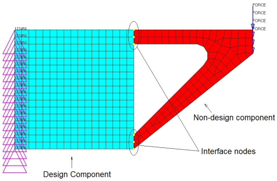
Figure 10. Example Model Indicating Design and Non-design Components and Boundary Nodes

First of all, a linear static analysis is performed on the complete structure. The displacement and von Mises stress results from this analysis (Figure 12).

Next, a reduced stiffness matrix and a load vector are generated for the non-design component. This is achieved by creating a new finite element model containing just the non-design component and the loads and boundary conditions directly applied to that component (Figure 11).

reduce_non_design
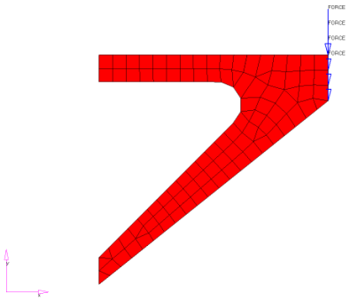
Figure 11. Reducing Out the Non-design Component

All of the degrees of freedom at the interface nodes (Figure 10) are selected as boundary degrees of freedom. ASET or ASET1 Bulk Data Entries are used to indicate this. The reduced matrices output is requested through the inclusion of the PARAM,EXTOUT,DMIGPCH Bulk Data Entry. The model is submitted to OptiStruct, resulting in the creation of the file filename_AX.pch which contains the reduced matrices in ASCII format. (Had PARAM,EXTOUT,DMIGBIN been used, the reduced matrices would be written in binary form to the file filename_AX.dmg).

The non-design component can now be replaced in the original model by its reduced matrix representation. This is done by manipulating the original model as:
  1. Delete the Bulk Data Entries for the nodes and elements of the non-design component.
  2. Delete all loads and boundary conditions that were only applied to the non-design component.
  3. Include the file containing the reduced matrices in the Bulk Data section.
  4. Select the reduced stiffness matrix with the Subcase Information Entry K2GG. (In this example, the reduced stiffness matrix will have the default name KAAX).
  5. Select the reduced load vector with the Subcase Information Entry P2G. (In this example, the reduced load vector will have the default name PAX).
Figure 13 shows the displacement and von Mises stress for the design component when the non-design component was replaced by a reduced matrix representation. It can clearly be seen, they match perfectly with the original model's results.


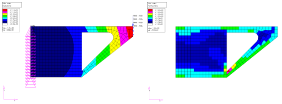
Figure 12. Results for a Linear Static Analysis on the Complete Structure (a) Displacements; (b) von Mises Stress


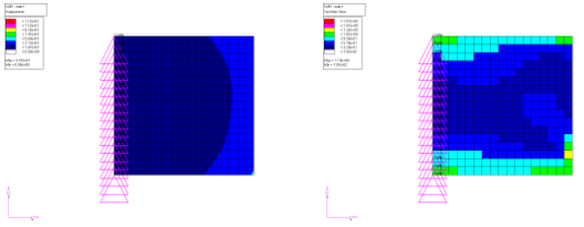
Figure 13. Results for a Linear Static Analysis with Reduced Matrix Substitution (a) Displacements; (b) von Mises Stress
Finally, for both the complete structural model and the reduced matrix model, a topology optimization was performed. For both models, the design component was identified as designable, the objective was to minimize the global compliance, and an upper limit of 50% was put on the volume fraction. The optimization results are shown in Figure 14.

dma3
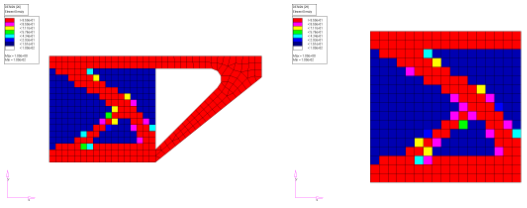
Figure 14. Density Results for a Topology Optimization (a) Complete Structure; (b) Reduced Matrix Substitution

Example 2: Static Condensation versus CBN

Figure 15 shows a finite element model running Normal Modes Analysis to compare the accuracy of static condensation and the dynamic condensation using CBN. The results are compared against the full model results.

The comparison clearly indicates that the dynamic reduction with CBN is highly accurate for this type of analysis, when compared to Static Condensation since the mass matrix is reduced accurately.

direct_matrix_superelement_model
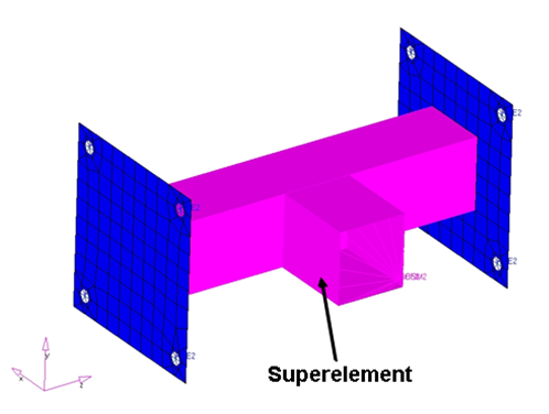
Figure 15. Normal Mode Analysis Model
Eigenmodes Full Model Static Reduction Dynamic Reduction (CMSMETH, CBN)
1 110.67 444.66 110.67
2 167.00 765.31 167.00
3 352.39 769.06 352.39
4 1272.95 2547.13 1272.96
5 1614.57 2923.56 1632.78

Component Dynamic Analysis (CDSMETH) Superelement Generation

The CDS superelement should be used when it is anticipated that a large number of residual runs will be made on a very large model at the higher end of the frequency range of study.

For example, this approach should be used when studying a variety of inputs on an automobile model in the frequency range of 400 to 800 Hz. For the residual analysis to run as fast as possible, all components, except very small ones, should be converted into CDS superelements. The major limitation of this approach is that it takes longer to generate the CDS superelements than with the other superelement creation methods. Also, the analysis must be performed at the fixed set of frequencies specified when the CDS superelement is formed. The major benefit of the CDS superelement is that the residual run will be much faster than with superelements created by other methods.

For an example of the body CDS superelement generation, see the input data for a body-in-white below. The special data for this input are the case control data: CDSMETH = 1; the FREQ card which restricts the residual analyses to just those frequencies; the CDSMETH data (see the CDSMETH card definition); and the BNDFREE data which defines the exterior points on the component.

CDS Body Super Element Example

MODEL = NONE
TITLE = BODY-IN-WHITE CDS MODEL
$-------------------------------------------------------------------------------
SUBCASE 1
FREQUENCY = 1
METHOD = 2
CDSMETH   = 1
BEGIN BULK
$==01==><==02==><==03==><==04==><==05==><==06==><==07==><==08==><==09==><==10==>
FREQ1          1     1.0     0.2      94
FREQ1          1    20.0     0.5     159
FREQ1          1   100.0     1.0      99
FREQ1          1   200.0     2.0     200
EIGRA          2          1000.0
CDSMETH        1

BNDFREE1 123456  1000000    through 1006001
INCLUDE '/MODELS/BODY/BODYNEW.dat'
ENDDATA

CDS superelement is saved in the file: XXX_CDS.h3d

The interface points (exterior points) are where the component is attached to another superelement directly or to the residual structure. These interface points must be independent degrees of freedom. If they are the dependent point of an RBE3, they must be made independent by transferring the dependencies to one of the independent grids referenced by the RBE3 element using UM data on the RBE3 definition, or use PARAM,AUTOMSET,YES. In the Bulk Data Entry section on the RBE3 element, the UM parameter shows how to redefine the dependency. The RBE3 can also be changed to an RBE2, but this could stiffen up the local area as a result.

In order to be formed into a superelement, a component FEA model has to be complete. All grids referenced in the superelement must be in the component model file. This includes local coordinate systems grids. All properties and material referenced in the components must also be included in the component. The component model must be able to be run successfully by itself in a modal analysis run.

The OSET field on the CDSMETH entry can be used to recover responses from the interior grids of the CDS superelements.

Residual Run Using the CDS Superelements

The residual run on the full model must be run with the direct analysis approach. Also, the same or a subset of the frequencies specified in the CDS superelement generation run must be used in the residual run.

The reduced matrices from CDSMETH will be used in residual run thru ASSIGN,H3DCDS. For CDSMETH, no DMIG selector entry such as K2GG is applicable but all the matrices in H3D file are used in residual run.

$ FOLLOWING CARD RETRIEVES THE H3D FILES FOR THE CDS SUPER ELEMENTS
ASSIGN,H3DCDS,AX,’myfile_CDS.h3d’
$
TITLE = P/T FULL VEHICLE ANALYSIS
SUBTITLE = FVM DIR H3D
SPC = 1
MPC =   406
SUBCASE 1
LABEL = UNIT LOAD INPUT INTO CDS MODEL
DLOAD = 110
FREQUENCY=1
SET 2 = 1006001,9106012
ACCELERATION (PUNCH,SORT2,PHASE) = 2
$
BEGIN BULK
$
$==01==><==02==><==03==><==04==><==05==><==06==><==07==><==08==><==09==><==10==>
FREQ1          1    1.0      0.2      94
FREQ1          1   20.0      0.5     159
FREQ1          1  100.0      1.0      99
FREQ1          1  200.0      2.0     200
EIGRL          1                   800.0   
$==01==><==02==><==03==><==04==><==05==><==06==><==07==><==08==><==09==><==10==>
$ 
INCLUDE  '/LOADS.dat'
$
INCLUDE  '/CONNECTIONS_BETWEEN_COMPONENTS.dat'
$   
INCLUDE  '/NON_CDS_COMPONENTS.dat'
ENDDATA