Seam Weld Fatigue Analysis
Seam Weld Fatigue analysis is available to facilitate Fatigue analysis for seam welded structures. It allows you to simulate the Fatigue failure at the seam weld joints to assess the corresponding fatigue failure characteristics like Damage and Life.
- Volvo Method (METHOD=VOLVO on FATPARM entry)
- Joint Line Method (METHOD=JNTLINE on FATPARM entry)
The Volvo method implemented in OptiStruct is based on a research paper Fatigue Life Prediction of MAG-Welded Thin-Sheet Structures published by M. Fermér, M Andréasson, and B Frodin. The method is a hot spot stress approach applicable to thin metal sheets. Hot spot stress is calculated from grid point forces at weld line. The method showed a good agreement with laboratory test results for sheet thickness between 1.0 mm and 3.0 mm. The method typically requires two SN curves. One is a bending SN curve which is dominated by bending stress, and the other is a membrane SN curve which dominated by membrane stress.
The Joint Line method is based on directly calculating the stresses within a certain evaluation distance from the joint or weld line. Additionally, unlike the Volvo method, the weld elements are not modeled in the Joint line method. The damage evaluation is only conducted at the root locations for Joint line method.
Implementation
Modeling Requirements: Volvo Method
- Weld sections to be analyzed for seam weld fatigue should be meshed with CQUAD4 elements whenever possible. CTRIA3 elements may be used for corner weld if inevitable and for closing the end of weld line, if necessary. Other element types are currently not supported for seam weld fatigue.
- The weld should be modeled by a single or double row of CQUAD4 elements. If a 2 sided fillet is to be modeled, a third row of CQUAD4 may be used.
- The thickness of the weld element is the same as the effective throat.
- The mesh size around the weld should be as regular as possible. Although this method is less sensitive to mesh size, a mesh size of about 10 mm would be a good choice according to Fermér, Andréasson, Frodin. This paper showed that large hot spot stress differences did not exist between mesh size 12 mm and mesh size 5 mm in case of a regular mesh.
- The weld element should have a dedicated property ID that is referenced by the PIDi fields of the FATSEAM Bulk Data Entry. For more information, refer to Input/Output. The property should be stiff enough to be a force transducer.
- The weld element normal direction should point outwards such that the normal direction is toward the weld toe, not toward the weld root. The normal direction of weld element plays a critical role in determining the weld toe and the surface to be examined on the base of the weld.
Modeling Requirements: Joint Line Method
- Unlike the Volvo method, the weld itself is not modeled in the Joint line method.
- The weld line or joint line should be represented using PLOTEL elements.
- These elements should be referenced as SETs on the ELSET continuation line of the FATSEAM Bulk Data Entry.
- Mismatch in mesh density is allowed on either side of the joint line.
- The normal direction of the shell elements part of the two or more plates welded at the joint line can be visualized in HyperMesh. The weld side (which side the Fatigue damage is evaluated) is determined based on the WLDSIDE field on the FATSEAM entry.
- All elements sharing the same weld line and REFEID should have consistent element normals, which match with the element normal identified by the corresponding REFEID element.
Weld Basics
- Face
- Toes
- Throat
- Root
- Legs

Figure 1. Basic Weld Structure
Good Weld Design Practice
This section provides a basic overview of stress concentrations in welded structures and a few recommendations for good weld design. This section should not be considered as a complete weld design guide and does not cover an exhaustive list of weld design recommendations.
- Weld shape-based stress concentration:Figure 2 shows the stress concentration at the toe of a weld. Its magnitude depends on the flank angle, , local weld toe radius, r, and plate thickness, t. The concept of a weld reinforcement is a misnomer as you can see that the stress concentration actually increases with increasing weld metal, that is, an increase in flank angle, .

Figure 2. Stress Concentration versus Weld Radius and Plate Thickness for Seam Weld Fatigue - Weld design-based stress concentration:
The second stress concentration comes from the joint design. Stress concentrations arise whenever there is a change in stiffness in the structure. It can result from either an increase of decrease in stiffness. For example, a hole in a plate will have about the same stress concentration as a rigid boss added to the plate. Here are some examples of weld joints contrasting good and poor design practice.
First you need to consider a cover plate welded to a bending beam. A large stress concentration exists at the end of the cover plate because of the large change in stiffness. A better design is shown on the right side where there is a more gradual change in stiffness.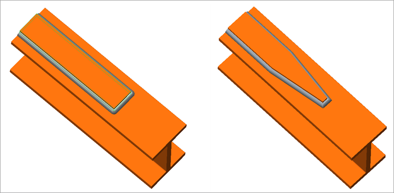
Figure 3. (a) Incorrect Weld Design; (b) Correct Weld Design: Gradual Stiffness GradientA second source of stress concentration is unintentional bending stresses caused by asymmetric geometries. The design on the left will have larger bending stresses than the double lap joint on the right side.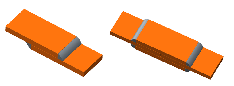
Figure 4. (a) Incorrect Weld Design; (b) Correct Weld Design: Double Lap Joint Symmetric GeometryWelding plates of differing thicknesses or widths is always problematic. Just as above, the easiest geometry to weld has the largest stress concentration. You should always consider moving the welds to lower stress areas in the structure and have a gradual transition in stiffness such as the joint shown Figure 5(b).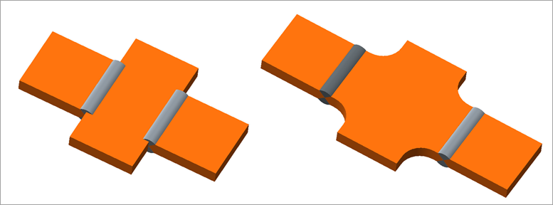
Figure 5. (a) Incorrect Weld Design; (b) Correct Weld Design: Gradual Stiffness Transition
Volvo Method
Supported Weld Types
OptiStruct supports certain types of welds for Seam Weld Fatigue Analysis.
- Only one row of elements can be defined for the weld face elements or either of the weld legs.
- The damage calculation locations are automatically chosen based on the weld type (as explained in Fillet). With the exception of the throat damage location, both the root and toe damage locations are evaluated based on the grid point forces and subsequent stresses induced in the corresponding elements adjacent to the weld elements. For throat damage, the weld element grid point forces, and subsequent stresses are directly considered.
- OptiStruct currently supports the following weld types.
Fillet

Figure 6. (a) Structure of a Fillet Weld; (b) T-Joint Seam Weld Element Representation
OptiStruct evaluates failures at root and toe when a weld element is CQUAD4. If CTRIA3 is used for a weld element, only toe is evaluated.
T-joint
- One-sided One RowFor a One-sided One Row T-joint, the weld element normal direction should point towards the weld toe. The nodes of the weld element are in line with the weld toes. The length should be determined by the actual dimensions of the weld element (typically L=T1+T2).

Figure 7. Representation of a One-sided T-Joint Fillet Weld with One Row of CQUAD4 ElementsThe thickness of the weld element is the effective weld throat (typically it is equal to L/1.414).
- One-sided Two RowMultiple rows are recommended for welds where the weld penetration is high and the weld typically forms the basis for contact between the two plates. Such welds are more rigid compared to welds where the penetration is lower, thereby additional rows of weld shell elements are required to capture the behavior. In Figure 8, the weld has penetrated more than the weld in Figure 7. For a One-sided Two Row T-joint, the two weld element normal directions should point towards the weld toe. The length should be determined by the actual dimensions of the weld element (typically L=T1+T2).

Figure 8. Representation of a One-Sided T-Joint Fillet Weld with Two Rows of CQUAD4 ElementsThe thickness of the weld element is recommended to be set equal to 0.35*L.
- Two-sided Two RowFor a Two-sided Two Row T-joint, the weld element normal directions should point towards the corresponding weld toe. The nodes of the weld elements are in line with the corresponding weld toes. The length should be determined by the actual dimensions of the weld element (typically L=T1+T2).

Figure 9. Representation of Two-Sided T-Joint Fillet Weld with Two Rows of CQUAD4 ElementsThe thickness of the weld element is the effective individual weld throat (typically it is equal to 1.414*L).
- Two-sided Three RowMultiple rows are recommended for welds where the weld penetration is high and the weld typically forms the basis for contact between the two plates. Such welds are more rigid compared to welds where the penetration is lower, thereby additional rows of weld shell elements are required to capture the behavior. In Figure 10, the welds have penetrated more than the welds in Figure 9. For a Two-sided Three Row T-joint, the two weld element normal directions should point towards the corresponding weld toe. The weld element normal for the central vertical element can point to either weld toe.

Figure 10. Representation of a Two-sided T-Joint Fillet Weld with Three Rows of CQUAD4 Elements
Cross-joint
- One-sided One RowFor a One-sided One Row Cross-joint, the weld element normal direction should point towards the corresponding weld toe.

Figure 11. Representation of a One-sided Cross-Joint Fillet Weld with One Row of CQUAD4 Elements Each - One-sided Two Row
Multiple rows are recommended for welds where the weld penetration is high and the weld typically forms the basis for contact between the two plates. Such welds are more rigid compared to welds where the penetration is lower, thereby additional rows of weld shell elements are required to capture the behavior. In Figure 12, the welds have penetrated more than the welds in Figure 11. For a One-sided Two Row Cross-joint, the weld element normal direction should point towards the corresponding weld toe. The vertical weld element normals should also point towards the corresponding weld toe.

Figure 12. Representation of a One-sided Cross-Joint Fillet Weld with Two rows of CQUAD4 Elements Each - Two-sided Two RowFor a Two-sided Two Row Cross-Joint, the weld element normal direction should point towards the corresponding weld toe.

Figure 13. Representation of a Two-sided Cross-Joint Fillet Weld with Two Rows of CQUAD4 Elements Each - Two-sided Three Row
Multiple rows are recommended for welds where the weld penetration is high and the weld typically forms the basis for contact between the two plates. Such welds are more rigid compared to welds where the penetration is lower, thereby additional rows of weld shell elements are required to capture the behavior. In Figure 14, the welds have penetrated more than the welds in Figure 12.
For a Two-sided Three Row Cross-Joint, the weld element normal direction should point towards the corresponding weld toe. The normals of the vertical weld elements can point towards either weld toe on each side.
Figure 14. Representation of a Two-sided Cross-Joint Fillet Weld with Three Rows of CQUAD4 Elements Each
Overlap or Laser Edge Overlap

Figure 15. Structure of an Overlap Weld
Meshing rules are the same as that for fillet weld. Normal direction of weld element should be toward weld toe. Weld nodes should be along the line of the weld toe. Weld element thickness should be effective weld throat. In laser weld, failure at weld throat is evaluated as well as weld toe and weld root.
Two Row Overlap
Multiple rows are recommended for welds where the weld penetration is high and the weld typically forms the basis for contact between the two plates. Such welds are more rigid compared to welds where the penetration is lower, thereby additional rows of weld shell elements are required to capture the behavior. The typical length of the weld element is L=T1+T2.

Figure 16. Representation of a Two Row Overlap Weld
One Row Overlap or One Row Laser Edge Overlap

Figure 17. Representation of a One Row Overlap Weld or Laser Edge Overlap Weld
One Row Overlap or One Row Laser Edge Overlap (Alternative)

Figure 18. Representation of an Alternative Approach for a One Row Overlap or Laser Edge Overlap
Laser Overlap

Figure 19. Representation of a Laser Overlap Weld
Failure Evaluation
Failure evaluation points differ from one weld type to another.

Figure 20. Attributes for Proper Identification of Entities
Fillet

Figure 21. Failure Locations for One Row Fillet

Figure 22. Failure Locations for Two Row Fillet
Overlap


Laser Overlap

Figure 26. Failure Locations for Laser Overlap
Laser Edge Overlap

Figure 27. Failure Locations for Laser Edge Overlap
Note the surface where weld throat is evaluated. This surface is determined by normal direction of the weld element.
Hot Spot Stress
OptiStruct calculates hot spot stress based on grid point force of a toe/root element.
In the original approach suggested by Fermér, Andréasson, Frodin, grid point forces contributed to the element of interest were directly used without any "adjustment". Later research [P. Fransson and G. Pettersson, 2000] showed that averaging grid point forces made grid point forces less mesh sensitive.
- OptiStruct identifies potential damage locations at weld toe, weld root, weld throat and their evaluation surface from weld elements location and its normal direction (as shown in previous sections).
- For the corresponding root and toe damage locations (in adjacent elements),
and in the throat (in the weld element), local coordinate systems are
constructed. The local X axis is constructed in the direction perpendicular
to and away from the corresponding weld element face at the center of the
adjacent element on the weld line (the X axis is in located in the plane of
the adjacent element). The local Y axis is constructed perpendicular to this
X axis in the plane of the adjacent element.

Figure 28. Seam Weld Stress Calculation Example - Grid point forces are calculated at grids (Q and R) of the adjacent element
(2) along the weld line. Grid point force contributions are sourced from
elements attached (1 and 3) to the adjacent element. Grid point forces are calculated as:
(1) (2) Moments are written as:(3) (4) - At each node ( and ) of the adjacent element that lies on the
weld line, averaged grid point forces/moments weighted by length of the
adjacent element and the attached element on the weld toe line are
calculated.Weighted forces are written as:
(5) (6) Weighted moments are written as:(7) (8) - Line Forces and Moments are calculated based on the weighted grid point
forces and moments. These line forces and moments from both ends of the
adjacent element on the weld line are averaged to generate the line force
and moment at the midpoint ().Line Forces are calculated as:
(9) (10) Line Moments are calculated as:(11) (12) The averaged line forces and moments at the midpoint, , for element 2 are:(13) (14) - The line force and moment at the midpoint are then resolved in the local coordinate system constructed in step 2 to generate and respectively. This force and moment pair leads to tensile and bending stresses in the adjacent element with respect to the weld line. These are the forces that are used to calculate stresses.
- Stresses are then calculated normal to the weld line for the adjacent
element from this force moment pair. Stresses are calculated for both top
and bottom of the shell element, and depending on the type of weld, either
one or both are used for fatigue calculations. This is the final hot spot
stress used in further S-N Fatigue Damage Evaluation. For addition
information, refer to Stress-Life (S-N) Approach.
(15) (16)
Fatigue Properties
There are a few fatigue properties relevant to Seam Weld Fatigue Analysis that allow you to control the fatigue behavior.
Bending Ratio

Figure 29. Example Stress Amplitude versus Fatigue Life log(N) for Bending dominated versus Membrane Dominated Structure
The upper and lower curves are referred to as Bending SN curve and Membrane SN curve, respectively. It is recommended that membrane SN curve should be used when membrane stress dominates in an element, and bending SN curve should be used when bending stress dominates. Interpolation between the two curves may be carried out depending on the degree of bending dominance.
- Maximum bending stress equal to
- Maximum membrane stress equal to
- Square of the maximum stress at the top surface of shell element at which the damage is calculated (that is, root, toe, or throat shell elements)
- Bending ratio of shell element .
is the
An interpolation factor () is now defined as:
when
when

Figure 30. Example Stress Amplitude versus Fatigue Life log(N) for Bending dominated versus Membrane Dominated structure
Thickness Correction
The thickness correction process is for size effect correction. SN curves are based on test results from a particular size of the specimen. In reality, the stress versus life curve may vary depending on specimen size. Therefore, thickness correction parameters can be used to correct for this effect. It may be applied based on the thickness of each shell element under consideration for Fatigue calculation (that is, toe, root, or throat element). The calculations are:
If , then there is no Thickness Correction.
This results in fatigue life reduction, making the design more conservative. TREF and TREF_N can be defined via the corresponding fields on the PFATSMW Bulk Data Entry. The default values are 1.0 and 0.2 respectively. The defaults are in inches (English units). If the metric system is used, then the values should be modified accordingly.
Thickness Correction can be turned on or off using the corresponding THCKCORR field on the FATPARM Bulk Data Entry for Seam Weld Fatigue Analysis.
Mean Stress Correction
FKM mean stress correction is supported for Seam Weld Fatigue. Stress sensitivity can be defined on the MATFAT Bulk Data Entry via the FKMMSS_SM field. Mean stress correction for Seam Weld fatigue is disabled by default and can be enabled via the corresponding CORRECT field on the FATPARM Bulk Data Entry.
Input/Output
To activate Seam Weld Fatigue Analysis, FATDEF has to have a FATSEAM and PFATSMW identifier.
Fatigue Element Identification
- The FATDEF Bulk Data and Subcase Information Entries can be used to identify the elements for which fatigue analysis should be performed. For seam weld fatigue, the FATSEAM and PFATSMW entries should be referenced on the FATDEF entry. The FATSEAM entry identifies the corresponding shell elements (CQUAD4 and CTRIA3) for which fatigue analysis is to be performed.
- The FATDEF Bulk Data Entry also provides the corresponding PFATSMW Bulk Data Entry references for each FATSEAM entry set to define the seam weld fatigue properties.
Fatigue Parameters
- The FATPARM Bulk Data and Subcase Information entries can be used to specify fatigue parameters for the seam weld fatigue analysis.
- The SMWLD continuation line on the FATPARM entry allows you to input the seam weld fatigue method and identify various parameters.
- The PFATSMW Bulk Data Entry allows the definition of some properties for seam weld fatigue analysis.
Fatigue Material
- The MATFAT Bulk Data Entry can be used to specify the material properties for seam weld fatigue analysis.
- The SMWLD continuation line allows you to specify mean stress sensitivity value, and separate SN curve attributes for bending and membrane SN curves. Bending SN curve and membrane SN curve may be defined in MATFAT after a flag SMWLD. If only one SN curve is defined for seam weld, it is used as both bending SN curve and membrane SN curve.
Fatigue Loads
- Similar to regular fatigue analysis, the FATLOAD, FATSEQ, and FATEVNT entries can be used to define loading sequences.
Optimization
- The PTYPE field on the DRESP1 entry can be set to FATSEAM and the ATTi fields should be FATSEAM identification numbers for seam weld fatigue optimization.
Output
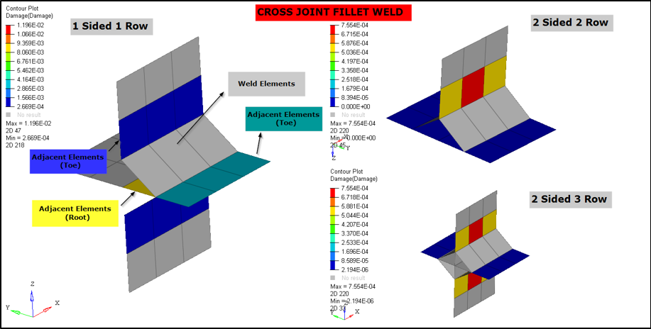
Figure 31. Example Cross Joint Fillet Weld Output for Damage
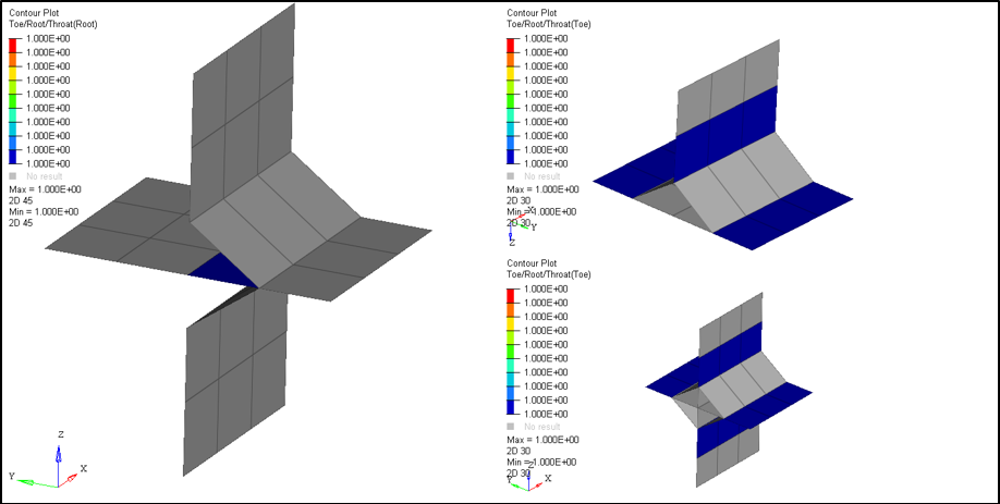
Figure 32. Example Cross Joint Fillet Weld Output for Toe/Root/Throat elements
Joint Line Method
Supported Weld Types
OptiStruct supports certain types of welds for Seam Weld Fatigue Analysis using the Joint Line method.
- The Weld elements should not be modeled when using the Joint Line method
- All elements sharing the same weld line and REFEID should have consistent element normals which match with the element normal identified by the corresponding REFEID element
- The damage calculation locations only consist of the toes of the welds and they are based on the evaluation distance (EVALDIS field on PFATSMW entry) as explained below.
- Refer to PFATSMW entry for more information on EVALDIS calculation
- OptiStruct currently supports the following weld
types for the Joint Line method.
WTYPE = L, T, GENERIC, BUTT
Fillet
A fillet weld is a weld joining two sheets at an angle. Two types of fillet weld are supported in Joint Line method (L, T). Fatigue calculation is conducted at the locations marked in yellow.
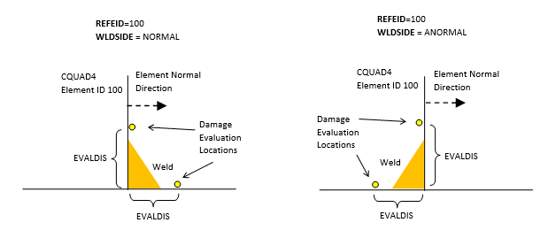
Figure 33. L-Fillet
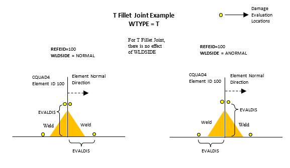
Figure 34. T-Fillet
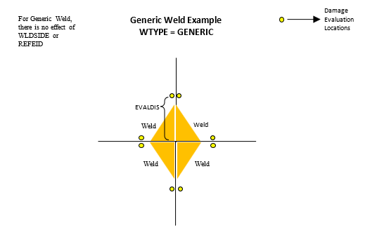
Figure 35. Generic Weld
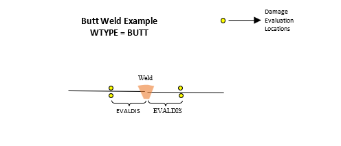
Figure 36. Butt Weld