Exercise 1: Linear Gap Analysis
Launch HyperMesh and Set the OptiStruct User Profile
Open the Model
Create a Cylindrical Coordinate System
-
In the Model Browser, click the Isolate
Shown icon
 .
.
-
Click the XY Top Plane View icon
 to set the model
view.
to set the model
view.
-
For xy plane, select any node on the plane of the lug, as shown in Figure 1:
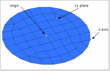
Figure 1. Nodes to Select for Creating Cylindrical Coordinate System -
Click the Card Editor icon
 .
.
-
Select the gap elements that are connected to the top lug, as shown in Figure 2.
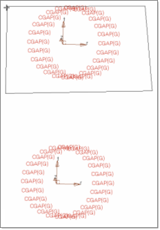
Figure 2. Gap Elements Connected to Top Lug -
Click CID, and select the system that was created at the
center of the top lug, as shown below.
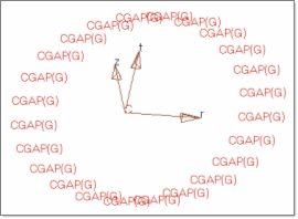
Figure 3.
Define a Property and Assign it to the Gap Elements
-
Make sure the check box next to KA_opts is checked. This determines the value
of KA for each gap element using the stiffness of surrounding elements
automatically.
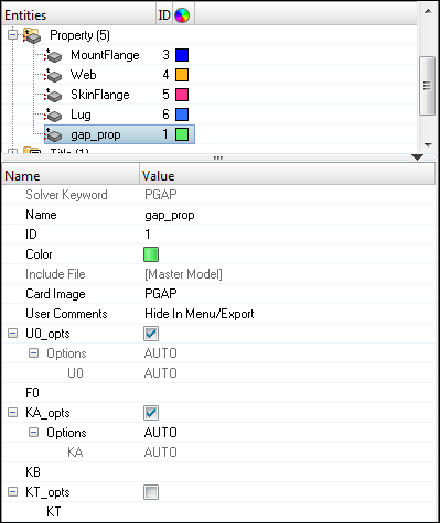
Figure 4.
Submit the Job
-
From the Analysis page, click the OptiStruct
panel.
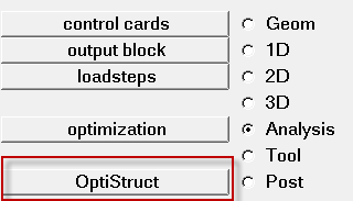
Figure 5. Accessing the OptiStruct Panel
The default files written to the directory are:
- rib_linear.html
- HTML report of the analysis, providing a summary of the problem formulation and the analysis results.
- rib_linear.out
- OptiStruct output file containing specific information on the file setup, the setup of your optimization problem, estimates for the amount of RAM and disk space required for the run, information for each of the optimization iterations, and compute time information. Review this file for warnings and errors.
- rib_linear.h3d
- HyperView binary results file.
- rib_linear.res
- HyperMesh binary results file.
- rib_linear.stat
- Summary, providing CPU information for each step during analysis process.
Post-process the Results
-
Click the Curves Attributes icon
 and hide all components except the Web component.
- Activate the Auto apply mode check box
- Click on the components to turn off in the modeling window
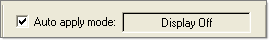
Figure 6. -
Go to the Contour panel
 .
.
-
Above the Results Browser in the left hand panel are the
Load Case and Simulation Selection drop-down menus. Select Subcase 1
(Coup_Vert) from the Load Case drop-down menu.
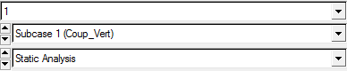
Figure 7. -
Click the XY Top Plane View icon to display a top view
of the Web.
-
Click Apply.
This should show the contour of stresses on the Web component under the coupled loading.
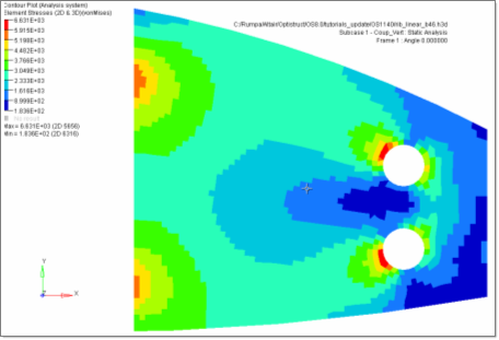
Figure 8. Stress Results on the Web From Linear Gap Analysis -
Click Delete Page
 to end the HyperView session.