結果
最適化コスト対反復計算のプロット
以下のプロットは、偏差が最小になるように最適化エンジンで設計が変更されるに伴って、コスト関数が減少する様子を示しています。
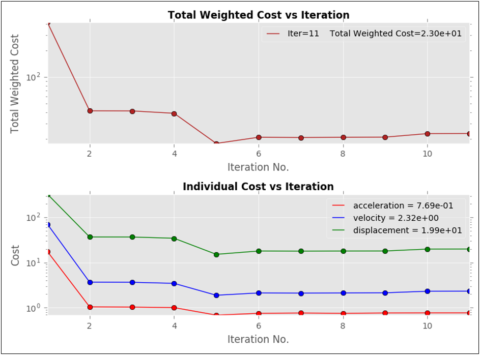
図 1.
注: y座標値は、小さい値を表示しやすくするために対数スケールでプロットされています。最適化エンジンでは11回の反復計算を必要としました。
図 1.
初期設計と最適化した設計の比較
初期設計と最適化した設計の両方について、このブロックの動的応答をプロットしています。変位、速度、および加速度が改善されています。
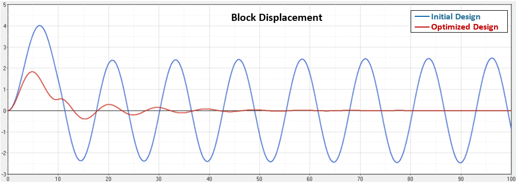
図 2.
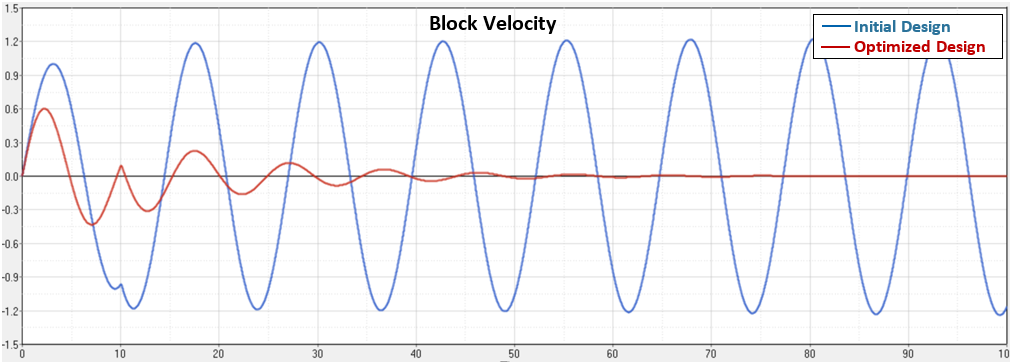
図 3.
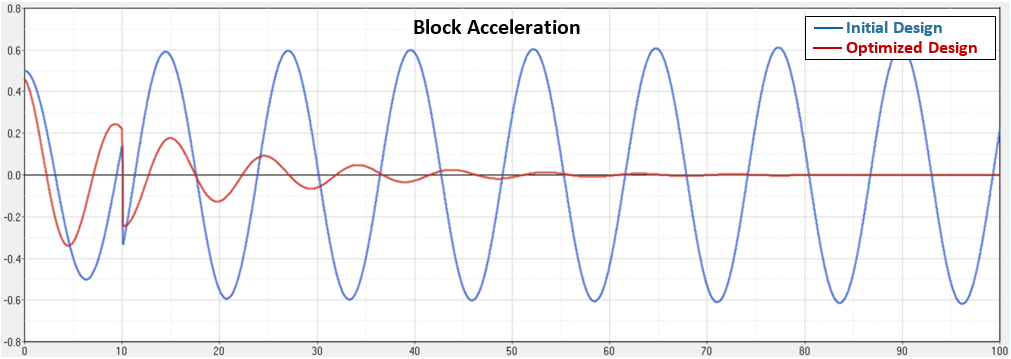
図 4.
図 2.
図 3.
図 4.
最適化のサマリーログファイル
OPTIMIZATION HISTORY FILE
Version 0.1


************************************************************************
**  COPYRIGHT (C) 2004-2016                 Altair Engineering, Inc.  **
** All Rights Reserved.  Copyright notice does not imply publication. **
** Contains trade secrets of Altair Engineering, Inc.                 **
** Decompilation or disassembly of this software strictly prohibited. **
************************************************************************

Date             : 14/03/2017
Time             : 17:09:18
Python Version   : 2.7.12 |Anaconda 4.2.0 (64-bit)| (default, Jun 29 2016, 11:07:13) [MSC v.1500 64 bit (AMD64)]

Input File       : c:\work\simulate function\pid.py
Output Directory : c:\work\simulate function\Two_Spring_with_force_170918
Summary File     : c:\work\simulate function\Two_Spring_with_force_170918\summary.log
Design Log File  : c:\work\simulate function\Two_Spring_with_force_170918\design.log

Optimizer Settings
------------------
Algorithm        : FMIN_SLSQP
Max. # iterations: 50
Accuracy         : 1.000e-03

Simulation Settings
-------------------
Analysis         : Call optimizer.sim_function
DSA              : FD

Iteration #   Cost #    Objective       Mag(Slope)
--------------------------------------------------
   1             6      4.1503e+02      1.3738e+04
   2            13      4.1491e+01      2.6595e+02
   3            24      4.1413e+01      1.8483e+02
   4            29      3.8928e+01      2.7961e+02
   5            34      1.7751e+01      6.9854e+01
   6            39      2.0843e+01      1.0056e+02
   7            49      2.0729e+01      1.8075e+02
   8            64      2.0828e+01      2.4888e+01
   9            79      2.0905e+01      2.2152e+02
  10            84      2.2928e+01      2.0147e+02
  11            89      2.3012e+01      7.2257e+01


Results from Optimization
-------------------------
Initial Cost   = 415.030
Final Cost     = 23.012
Cost reduction = 94.455

Individual Responses
--------------------
Weight = 1.00 Final cost of objective acceleration = 0.77
Weight = 1.00 Final cost of objective velocity = 2.32
Weight = 1.00 Final cost of objective displacement = 19.92

Final Design Table
------------------

DV                Lower Bound        Upper Bound        Initial Value      Optimized Value
------------------------------------------------------------------------------------------
DV0               +0.0000e+00        +1.0000e+00        +0.0000e+00        +1.5952e-01
DV1               +0.0000e+00        +1.0000e+00        +5.0000e-01        +8.7677e-01
DV2               +0.0000e+00        +1.0000e+00        +0.0000e+00        +4.5369e-01

Elapsed Time for job                       = 261.13 seconds
  Time in Cost function                    = 130.75 seconds
  Time in Sensitivity function             = 124.84 seconds


Optimization process completed.
設計のサマリーログファイル
Design History
Input File      : c:\work\simulate function\pid.py
Output Directory: c:\work\simulate function\Two_Spring_with_force_170918

Iteration #   Design
--------------------------------------------------------------------------------

   1          [0.0, 0.5, 0.0]
   2          [0.27699, 0.63833, 2.3762e-05]
   3          [0.27832, 0.63779, 2.3718e-05]
   4          [0.2731, 0.6548, 3.3886e-12]
   5          [0.076768, 1.0, 0.64752]
   6          [0.13338, 0.91154, 0.44929]
   7          [0.13338, 0.9115, 0.44932]
   8          [0.13338, 0.9115, 0.44932]
   9          [0.13338, 0.9115, 0.44932]
  10          [0.15857, 0.87803, 0.45354]
  11          [0.15952, 0.87677, 0.45369]