Flux Panel
Use the Flux panel to apply concentrated fluxes to your model. This is accomplished by applying a load, representing fluxes, to element nodes. Fluxes are load config 6 and are displayed as a thick arrow labeled with the word "flux."
Location: Analysis page
Loads from files formatted as CSV (Comma Separated Values) or SSV (Space-Separated Values) text files can be interpolated.
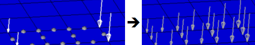
Field Loads will not overwrite any existing loads, so you can create an area of loads via linear interpolation and then use field loads to expand the load area without changing the loads already inside of the area.
Create Subpanel
| Option | Action |
|---|---|
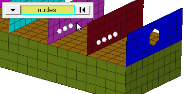
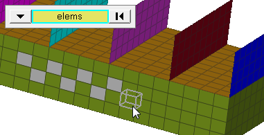
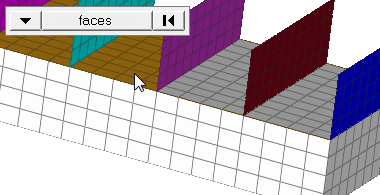
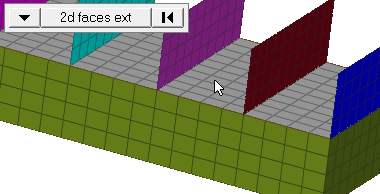
| entity selector | Select the type of entity that you wish to pick. In
any case, the fluxes are applied to nodes; this choice simply determines how
those nodes are selected. Elems select the nodes at the corner of each element
picked. Geometric points select the nodes at which they exist. Comps select all
of the nodes contained within the chosen component or set. If you choose comps
or sets, the loads are drawn using a single indicator. As a result, a new button
called display appears. This allows you to indicate where in the model you wish
the indicator to be drawn, and requires additional steps. When you select nodes or
elems, click the switch to change the selection mode.
|
| value |
|
| relative size / uniform size |
By default, loads are displayed relative to the model
size.
Note: This setting does not affect the flux load, only the
length of its graphical indicators.
|
| label loads | Display the load's text labels in modeling window. |
| load types | Select a load type. |
| face angle / individual selection |
|
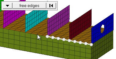
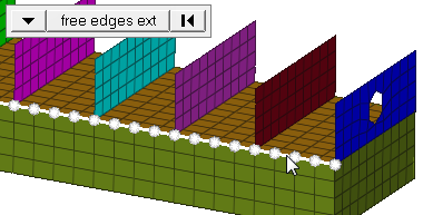
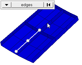
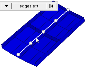
| edge angle |
Split edges that belong to a given face. When the edge
angle is 180 degrees, edges are the continuous boundaries of faces. For smaller
values, these same boundary edges are split wherever the angle between segments
exceeds the specified value. A segment is the edge of a single element.
Important: Only available when the entity selector is set to nodes and the
selection mode is set to free edges, free edges ext, edges, or edges
ext.
|
Update Subpanel
| Option | Action |
|---|---|
| entity selector | Select the type of entity that you wish to pick. In any case, the fluxes are applied to nodes; this choice simply determines how those nodes are selected. Elems select the nodes at the corner of each element picked. Geometric points select the nodes at which they exist. Comps select all of the nodes contained within the chosen component or set. If you choose comps or sets, the loads are drawn using a single indicator. As a result, a new button called display appears. This allows you to indicate where in the model you wish the indicator to be drawn, and requires additional steps. |
| value |
|
| relative size / uniform size |
By default, loads are displayed relative to the model
size.
Note: This setting does not affect the flux load, only the
length of its graphical indicators.
|
| label loads | Display the load's text labels in modeling window. |
| load types | Select a load type. |
Command Buttons
| Button | Action |
|---|---|
| create | Create the load. |
| create/edit | Create the load and open the card image for editing. |
| reject | Revert the most recent changes. |
| review | Review the load in the modeling window. |
| update | Update the load with the most recent changes. |
| return | Exit the panel. |
Equations allow you to create force, moment, pressure, temperature or flux loads on your model where the magnitude of the load is a function of the coordinates of the entity to which it is applied. An example of such a load might be an applied temperature whose intensity dissipates as a function of distance from the application point, or a pressure on a container walls due to the level of a fluid inside.
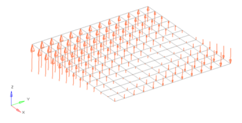
Figure 14. Flat Plate with a Linear Function for an Applied Force Magnitude = 20 – (5*x+2*y). The flat plate is 20 x 20 units, lying in the X-Y plane with the origin at the center.
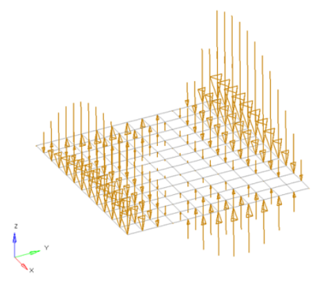
Figure 15. Flat Plate with a Polynomial Function with Magnitude = x^2-2y^2+x*y+x+y. The flat plate is 20 x 20 units, lying in the X-Y plane with the origin at the center.
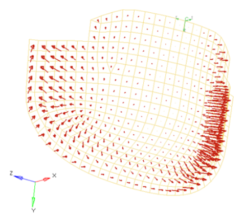
Figure 16. Curved Surface with a Polynomial Function for an Applied Pressure Magnitude = -((x^2+2*y^2+z)/1000). The pressure function is defined in terms of the cylindrical coordinate system displayed at the top edge of the elements.