Temperatures Panel

Use the Temperatures panel to create temperature constraints.

Location: Analysis page

Temperatures constraints are created by applying a load that represents temperatures to nodes, components surfaces, sets, points, or lines.

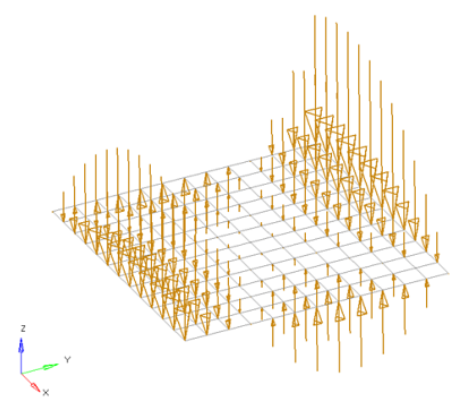
Temperatures are load config 5 and are displayed as a vertical line with the letter T at the top.

Create Subpanel

Option	Action
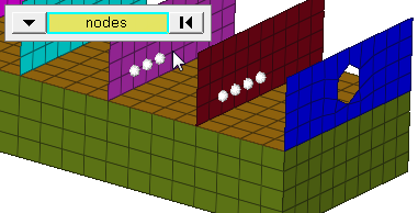
entity selector	Select entities to which temperatures will be applied. In any case, the forces are applied to nodes; this selection simply determines how those nodes are selected. Geometric points select the nodes at which they exist. Comps select all of the nodes contained within the chosen component. When nodes is selected, use the switch to change the selection mode. nodes Select individual nodes. Figure 1. 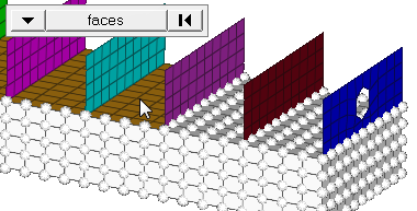Example: Nodes Selection faces Select all of the nodes on 2D and 3D faces. If there are discontinuities on a 2D face, then only the nodes inbetween the discontinuities will be selected. Figure 2. 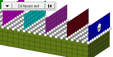Example: Faces Selection 2D faces ext Select all of the nodes on a 2D face that contain discontinuities. Figure 3. 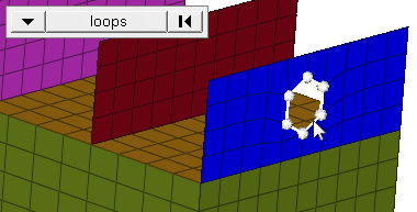Example: 2D Faces Ext Selection loops Select all of the nodes on continuous free edges that make a closed loop simultaneously, such as the perimeter of a hole. Important: Only valid for SHELL elements. Figure 4. 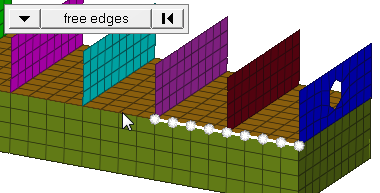Example: Loops Selection free edges Select all of the nodes on free edges of elements. If there are discontinuities on an edge, then only the nodes on the free edges inbetween the discontinuities will be selected. Important: Only valid for SHELL elements. Figure 5. 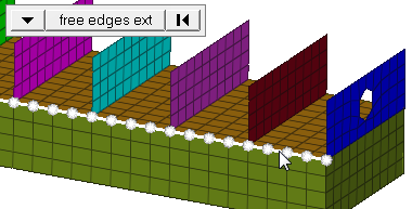Example: Free Edges Selection free edges ext Select all of the nodes on free edges of elements that contain discontinuities. Important: Only valid for SHELL elements. Figure 6. 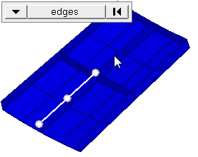Example: Free Edges Ext Selection edges Select all of the nodes on free edges or shared edges (butt joints, L/corner joints, and T-joints) of elements. If there are discontinuities on an edge, then only the nodes on the edge inbetween the discontinuities will be selected. Important: Only valid for SHELL elements. Figure 7. 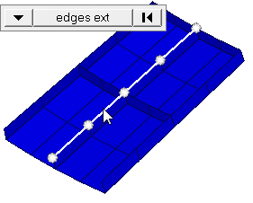Example: Edges Selection edges ext Select all of the nodes on free edges or shared edges (butt joints, L/corner joints, and T-joints) of elements that contain discontinuities. Important: Only valid for SHELL elements. Figure 8. Example: Edges Ext Selection
value =	constant value The value of the load magnitude. constant components Specify the direction and magnitude of the load by entering the X, Y, and Z values of the components. curve, vector When working with loads that are time-dependent, specify the time history of the load using a vector entity. When using this option, you may choose to apply the load normal to the elements, or use the plane and vector selector to specify a direction. Use the curve selector to select the curve representing the load time history. This curve must already exist in the model. The optional scale factor field allows you to scale the X vector of the curve. Curves can be viewed and modified from within the XY Plots module. curve, components Specify the X, Y, and Z components to define the direction and magnitude, for example, (2,2,2) will be twice the magnitude of (1,1,1). Next, double-click curve to select an existing curve. Last, specify a factor for the curve’s xscale to use the same curve for many different cases, but vary the scale of its intensity or time to match the needs of your current load. equation Specify the loading equation^¹. Use the plane and vector selector to specify a direction, then select the coordinate system to which the vector corresponds. 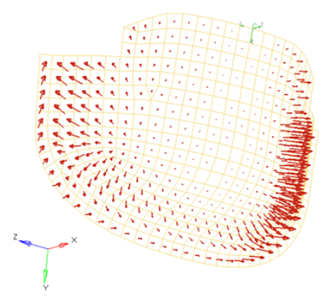linear interpolation Interpolate loads from a saved file or existing loads. Note: Only available for shell elements. Each row of the input file contains the x,y,z coordinates of the load followed by its three components. The data can be separated by a space or tab. You can then select the desired nodes to which you wish to add loads, and pick 3 or more existing loads that enclose those nodes. When you interpolate, a linear function is used to create additional loads on the selected nodes, with magnitudes based on the magnitudes of the loads that you had selected. Figure 9. In the search radius field, specify the search distance to find the loads which are within that distance from a centroid or node on which a load is being interpolated. The nearest 3 loads located within that distance are used to create the load at the centroid or node by linear interpolation. Linear interpolation uses a triangulation method, so if it finds fewer than 3 loads within that distance no interpolation takes place. While reading the initial loads from a file, if linear interpolation is not possible because the search radius is too small, the original loads are simply applied to the nearest centroid or node. Select fill gap to create a load at every selected element centroid or node irrespective of the size of the search radius. field loads Interpolate and extrapolate loads from existing loads. You can then select the desired elements to which you wish to add loads, and any existing loads on which you wish to base additional forces. When you create, Engineering Solutions uses a Green's function with the given boundary loads in order to create the loads on all of the selected nodes. For smoothness, the gradient at the boundary points is enforced to be zero; this ensures that the extrapolated loads remain lower than the input loads. For this reason it is recommended to use representative boundary values as input to be able to capture the peaks reasonably. Note: This version differs from linear interpolation both in the way that the load magnitudes are determined, and also in the fact that it can be applied to nodes outside the boundaries of the chosen existing loads.
relative size / uniform size	By default, loads are displayed relative to the model size. relative size= Display loads in a size relative to the model size (default 100). uniform size= Display all loads with the same size.
label loads	Display the load's text labels in modeling window.
load types	Select a load type.
face angle / individual selection	face angle Determines which of the selected support entities will have the panel entity (ex: load, boundary condition, vector, set definition, and so on) applied. The face angle value is used to determine which faces will be selected based on the angle difference between the selected and adjacent face normals. If the angle between the normals of the faces is less than this face angle value the face is included. This process is similar for edge selection, except that the angle between edges is used instead of the angle between faces. Important: Only available when the entity selector is set to nodes, and the selection mode is set to faces, 2d faces ext, free edges, free edges ext, edges, or edges ext. individual selection Select individual elements on a face or select individual free/shared edges of elements. Important: Only available when the entity selector is set to nodes and the selection mode is set to faces, free edges, or edges.
edge angle	Split edges that belong to a given face. When the edge angle is 180 degrees, edges are the continuous boundaries of faces. For smaller values, these same boundary edges are split wherever the angle between segments exceeds the specified value. A segment is the edge of a single element. Important: Only available when the entity selector is set to nodes and the selection mode is set to free edges, free edges ext, edges, or edges ext.

Update Subpanel

Option	Action
loads	select the loads to modify.
value =	constant value The value of the load magnitude. constant components Specify the direction and magnitude of the load by entering the X, Y, and Z values of the components. curve, vector When working with loads that are time-dependent, specify the time history of the load using a vector entity. When using this option, you may choose to apply the load normal to the elements, or use the plane and vector selector to specify a direction. Use the curve selector to select the curve representing the load time history. This curve must already exist in the model. The optional scale factor field allows you to scale the X vector of the curve. Curves can be viewed and modified from within the XY Plots module. curve, components Specify the X, Y, and Z components to define the direction and magnitude, for example, (2,2,2) will be twice the magnitude of (1,1,1). Next, double-click curve to select an existing curve. Last, specify a factor for the curve’s xscale to use the same curve for many different cases, but vary the scale of its intensity or time to match the needs of your current load. equation Specify the loading equation^¹. Use the plane and vector selector to specify a direction, then select the coordinate system to which the vector corresponds. linear interpolation Interpolate loads from a saved file or existing loads. Note: Only available for shell elements. Each row of the input file contains the x,y,z coordinates of the load followed by its three components. The data can be separated by a space or tab. You can then select the desired nodes to which you wish to add loads, and pick 3 or more existing loads that enclose those nodes. When you interpolate, a linear function is used to create additional loads on the selected nodes, with magnitudes based on the magnitudes of the loads that you had selected. Figure 10. In the search radius field, specify the search distance to find the loads which are within that distance from a centroid or node on which a load is being interpolated. The nearest 3 loads located within that distance are used to create the load at the centroid or node by linear interpolation. Linear interpolation uses a triangulation method, so if it finds fewer than 3 loads within that distance no interpolation takes place. While reading the initial loads from a file, if linear interpolation is not possible because the search radius is too small, the original loads are simply applied to the nearest centroid or node. Select fill gap to create a load at every selected element centroid or node irrespective of the size of the search radius. field loads Interpolate and extrapolate loads from existing loads. You can then select the desired elements to which you wish to add loads, and any existing loads on which you wish to base additional forces. When you create, Engineering Solutions uses a Green's function with the given boundary loads in order to create the loads on all of the selected nodes. For smoothness, the gradient at the boundary points is enforced to be zero; this ensures that the extrapolated loads remain lower than the input loads. For this reason it is recommended to use representative boundary values as input to be able to capture the peaks reasonably. Note: This version differs from linear interpolation both in the way that the load magnitudes are determined, and also in the fact that it can be applied to nodes outside the boundaries of the chosen existing loads.
relative size / uniform size	By default, loads are displayed relative to the model size. relative size= Display loads in a size relative to the model size (default 100). uniform size= Display all loads with the same size.
label loads	Display the load's text labels in modeling window.
load types	Select a load type.

Command Buttons

Button	Action
create	Create the new load.
create/edit	Create the new load and open its property card in edit mode.
reject	Revert the most recent load creation.
review	Click review, then select the temperatures to review on your model. After you select each temperature, the value of the temperature is displayed.
update	Change the selected load(s) to use the currently-specified characteristics.
return	Exit the panel.

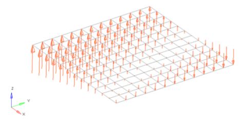
Equations allow you to create force, moment, pressure, temperature or flux loads on your model where the magnitude of the load is a function of the coordinates of the entity to which it is applied. An example of such a load might be an applied temperature whose intensity dissipates as a function of distance from the application point, or a pressure on a container walls due to the level of a fluid inside.

Functions must be of the form magnitude= f(x,y,z). The only variables allowed are x, y and z, (lower case) which are substituted with the coordinate values of the entity to which the load is applied. In the case of grid point loads (force, moment or temperature) the grid point coordinates are used. For elemental loads (pressure or flux) the element centroid coordinates are used. In the event that a cylindrical or spherical coordinate system is used, x, y and z are still used to reference the corresponding direction. Standard mathematical operators and functions can be used; however, any functions requiring external data will not be valid.

Note: If your equation contains a syntax error, no warning message will be displayed, but any loads created will have a zero magnitude.